Intro

In this post I’ll try to describe one of my favorite “weekend projects”. Although it took almost a month to finish, I still call it a weekend project because I never used it for any senior research.

Since I graduated in Electrical Engineering, I always wanted to simulate what I think is THE most fundamental system of equations for us (Electrical Engineers): The Maxwell’s equations. A couple of years back I finally had time to do so, and I’ll share with you the work I did. Everything is on GitHub, so if you want to try yourself, please feel free to fork the repository and play around!

In this post I’ll assume that you have at least a vague idea of what Maxwells equations are and that they describe how electromagnetic fields behave. Also, I assume that you know that light is a “moving electromagnetic field” (called electromagnetic wave). So, if we are able to describe and simulate electromagnetic waves, we can actually describe and simulate light!

Before show the simulations, let me start with a bit of explanation about the electromagnetic theory. The most obvious place to start is with Maxwell’s equations themselves: $$ \begin{equation} \begin{gathered} \nabla \cdot \vec E = \frac{\rho }{{{\varepsilon _0}}} \hfill \\ \nabla \cdot \vec B = 0 \hfill \\ \nabla \times \vec E = – \frac{{\partial \vec B}}{{\partial t}} \hfill \\ {c^2}\nabla \times \vec B = \frac{{\vec J}}{{{\varepsilon _0}}} + \frac{{\partial \vec E}}{{\partial t}} \hfill \\ \end{gathered} \end{equation} $$ These equations together with a couple of technical details like continuity constraints and boundary conditions, simply describes ALL physics related to electromagnetic fields. That includes radio waves, light, electricity, magnetism and etc. It is not the goal of this post to talk about Maxwell’s equation themselves, but rather about its solutions. In particular, about numeric solutions. Also, I do not intend to go deep into the theory of the simulation method, but rather to show its potential and encourage you to try! This post is not a tutorial, but I’ll try to point you in the right direction if you want to do it yourself. Also, I have to assume that you know some Calculus (at some not so basic level, I’m afraid).

First of all, lets understand what a solution to Maxwell’s equation means. Any equation that describes a physical phenomenon is a kind of mathematical description of that phenomenon. For instance, the famous Newton’s equation $F = m\,a$ tells us that if you have a mass of $10Kg$ and it is accelerating with an acceleration of $2m/s^2$, there should be a force of $20N$ being applied to the mass. In the same way, Maxwells equation tells us that if a medium has electrical permittivity $\varepsilon_0$, the charge density is $\rho$, etc, etc, then the electric and magnetic fields MUST be such that the divergent of the electric field is $\rho / \varepsilon_0 $ and etc. For instance, Maxwell’s equation directly states that, whatever the situation is, the divergent of the magnetic field is zero. And so on…

So, that means that if you know the environment, in another words, you know how its permittivity, permissively, charge density, etc are distributed, you can predict how the electromagnetic fields will behave on this environment. In order to do that, you solve Maxwell’s equations to find ${\vec E}$ and ${\vec B}$.

It turns out that Maxwell’s equations, although they have a “simple” look, they are kind of “extensive” in the sense that the electric and magnetic fields have each one 3 components x, y and z and each component varies in space and time. Also they are partial differential equations, which involve all the derivatives of the solution either in x, y, z and t! So, to solve the Maxwell’s equation mean to find 6 functions of 4 variables. In general that is not possible to do analytically except in special cases. Hence, we have to appeal to numeric solutions. There are tons of methods for numerically solve a partial differential equation. In this post we will talk about the FD-TD method (due to Kane S. Yee) or method of Finite Diferences in the Time Domain (sometimes called Yee method). The method itself is pretty straightforward and, as all numerical method, it begins by exchanging the functions themselves by a grid of discrete values. As I mention, I won’t go deep into the method itself, but I’ll try to give an idea of how it works. Another important thing: I implemented the 2D version of the FD-TD method. So, the simulation will consist in a fields that is the same in the z direction form minus infinity to infinity. Unfortunately, cool things like polarization of light won’t be possible here (by definition, a 2D wave is aways polarized). But don’t worry, I promise that you can still have A LOT of fun with this apparently frustrating limitation.

In summary up to now, we will solve Maxwell’s equation numerically using the FD-TD method. So, what does this mean in practice? That means that we are going to divide our environment in a grid (2D for our case) and set each point on the grid with objects like conductors, sources, walls and etc. After that, we compute the electric and magnetic field on each point on the grid at each instant of time. The result is that, hopefully, we are going to see an “animation” of the fields interacting with our small “world”. Figure 1 tries to show a possible setup for a simple simulation.

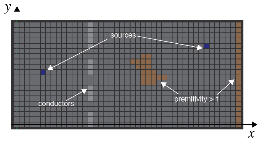
Figure 1: 2D grid with a source of electric field and some objects with different permittivities conductivities.

The FD-TD method itself[1] is well described in lots of places, books, etc. But if I were to recommend a place where you can learn very well, I would recumbent the youtube channel CEM lectures[2]. I saw some videos on FD-TD method and they are really good!

Finite-Difference Time-Domain method

Here I’ll briefly describe the idea behind the method itself. The idea is based on the approximation of the derivatives by differences divided by the step. This principle is very well suited for ordinary differential equations that approximates derivatives in time. $$ \begin{array}{l} \frac{{dx(t)}}{{dt}} \approx \frac{{x(t + \Delta t) – x(t)}}{{\Delta t}}\\ x(t + \Delta t) \approx x(t) + \frac{{dx(t)}}{{dt}}\Delta t \end{array} $$ The time portion of the method is called “leapfrog” step and is based on this idea of integrating the time derivative. As you can see, it provides a way of computing the next value of the function $x(t+\Delta t)$ used on its current values $x(t)$. This is also called Euler’s method. In the FD-TD, method, the time derivative also depends on the derivative in space. Since we will focus on the 2D version, one of the fields (either the electric or the magnetic) will be the same in the z direction (z here is arbitrary). Depending on which you choose to be constant in the z direction, we call the setup as TE or TM (transverse electrical or transverse magnetic). All derivatives in z will be zero for the chosen field and it will not have x and y components. The other field then won’t have the z coordinate, only x and y. The reason this happens is that the curl of the field is a intrinsic 3D operation. In fact, although we simulate in a 2D world (even 1D for that matter) the fields are still three dimensional entities. What happens is that some components are zero or remans constant from minus infinity to infinity.

There is still one “trick” that must be done in the numerical setup for the FD-TD method. Since se have relationships with the curl of the fields, we have to consider the resulting vector to the in the “center” of the diferences. So, in the TM approach, the electric field have to be in the center of the magnetic fields (and no magnetic field must be present). So, for the method to work, we have to “stagger” the grid, moving it “half step” in x and y for one of the fields. So, this produces a grid for the electric field that is halfway displayed from the magnetic field. This is important for the assignment of the spacial indices for the electric and magnetic fields. Figure 2 shows the staggered grid that represents the electric and magnetic fields in the TM configuration.

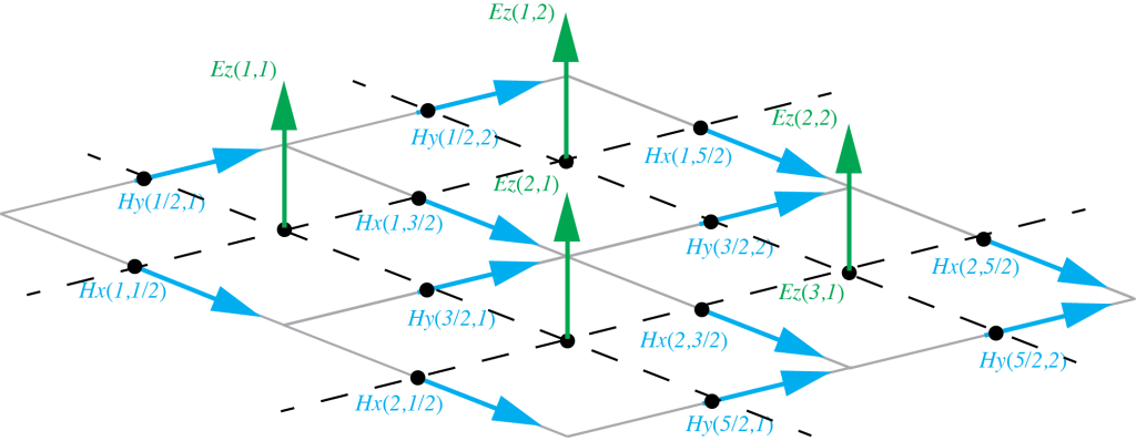
Figure 2: Staggered grid for the electric and magnetic fields in the TM scenario

As you can see, the staggered grid trick forces the electric field be always surrounded by magnetic field. This is perfect to approximate the curl equation. As a practical note, the “half” spatial step is just a notation stunt. In the end, in the computer, it will be all integer indices. This notation makes it easy to locate each field in the discrete approximation.

Since we dealing with the 2D simulation, this simplifies the difference equations for the whole set of Maxwell’s equations. In fact we end up with this set of difference equations[3] bellow. Observe that the order of computation here matters… This is a technical detail that has to do with the stability of the method. Since we are integrating, if we do not compute things right, we might generate a systematic error in one of the fields, causing it to integrate more then necessary and blow up the values. $$ \begin{array}{l} {H_x}\left[ {m,n + \frac{1}{2},q + \frac{1}{2}} \right] = {H_x}\left[ {m,n + \frac{1}{2},q – \frac{1}{2}} \right] – \\ \frac{{\Delta t}}{{\mu \Delta y}}\left( {{E_z}\left[ {m,n + 1,q} \right] – {E_z}\left[ {m,n,q} \right]} \right) \end{array} $$ $$ \begin{array}{l} {H_y}\left[ {m + \frac{1}{2},n,q + \frac{1}{2}} \right] = {H_y}\left[ {m + \frac{1}{2},n,q – \frac{1}{2}} \right] + \\ \frac{{\Delta t}}{{\mu \Delta x}}\left( {{E_z}\left[ {m + 1,n,q} \right] – {E_z}\left[ {m,n,q} \right]} \right) \end{array} $$ $$ \begin{array}{l} {E_z}\left[ {m,n,q + 1} \right] = \frac{{2\varepsilon – \rho \Delta t}}{{2\varepsilon + \rho \Delta t}}{E_z}\left[ {m,n,q} \right] + \\ \frac{{2\varepsilon }}{{2\varepsilon + \rho \Delta t}}\left( \begin{array}{l} \frac{{\Delta t}}{{\varepsilon \Delta x}}\left( {{H_y}\left[ {m + \frac{1}{2},n,q + \frac{1}{2}} \right] – {H_y}\left[ {m – \frac{1}{2},n,q + \frac{1}{2}} \right]} \right)\\ – \frac{{\Delta t}}{{\varepsilon \Delta y}}\left( {{H_x}\left[ {m,n + \frac{1}{2},q + \frac{1}{2}} \right] – {H_x}\left[ {m,n – \frac{1}{2},q + \frac{1}{2}} \right]} \right) \end{array} \right) \end{array} $$ Now let me just comment a bit about the notation. $E_z[m,n,q]$ is the electric field in z at index m and n in the grid at instant q in time (same for the other fields). $\rho$, $\epsilon$ and $\mu$ are the conductivity, permittivity and permeability of the medium. Although not explicitly in the equations, each one also depend on the position on the grid m and n ($\rho[m,n]$, $\epsilon[m,n]$ and $\mu[m,n]$). The deltas are the spacing for the discretization in space and time.

Actually, the “algorithm” of FD-TD is pretty much only that! Its a loop that keeps updating the fields according to those equations. The heart of the implementation is the step that do that update. The code is as simple as this one

function [Ezo, Hxo, Hyo] = leapFrog2D(Ezi, Hxi, Hyi, parameters)

    Ezo = Ezi;
    Hxo = Hxi;
    Hyo = Hyi;


    c1 = parameters.c1;
    c2 = parameters.c2;
    c3 = parameters.c3;
    c4 = parameters.c4;
    dx = parameters.dx;
    dy = parameters.dy;
    boundary = parameters.boundary; 
    wire = parameters.wire;
    
   
    Nx = size(Ezi,1);
    Ny = size(Ezi,2);
    
    j_p_0_E = 1:Nx-1;
    j_p_0_E = 1:Ny-1;

    i_p_1_E = 2:Nx;
    j_p_1_E = 2:Ny;

    i_p_0_H = 1:Nx-1;
    j_p_0_H = 1:Ny-1;

    i_p_1_H = 2:Nx;
    j_p_1_H = 2:Ny;

   
    % transverse electric
  
    Ezo(i_p_1_E, j_p_1_E) = c1(i_p_1_E, j_p_1_E).*Ezi(i_p_1_E, j_p_1_E) + c2(i_p_1_E, j_p_1_E).*(  ( wire(i_p_1_E, j_p_1_E).*Hyi(i_p_1_E, j_p_1_E) - wire(i_p_0_E, j_p_1_E).*Hyi(i_p_0_E, j_p_1_E) )/dx - ( wire(i_p_1_E, j_p_1_E).*Hxi(i_p_1_E, j_p_1_E) - wire(i_p_1_E, j_p_0_E).*Hxi(i_p_1_E, j_p_0_E) )/dy   );

    Hxo(i_p_0_H, j_p_0_H) = Hxi(i_p_0_H, j_p_0_H) + c3(i_p_0_H, j_p_0_H).*(   ( wire(i_p_0_H, j_p_0_H).*Ezo(i_p_0_H, j_p_0_H) - wire(i_p_0_H, j_p_1_H).*Ezo(i_p_0_H, j_p_1_H) )/dy   );
    Hyo(i_p_0_H, j_p_0_H) = Hyi(i_p_0_H, j_p_0_H) + c4(i_p_0_H, j_p_0_H).*(   ( wire(i_p_1_H, j_p_0_H).*Ezo(i_p_1_H, j_p_0_H) - wire(i_p_0_H, j_p_0_H).*Ezo(i_p_0_H, j_p_0_H) )/dx   );
end

The whole code is in GitHub[4]. As you can see, its the implementation of the update equations. This function keeps being called in a loop. The “heavy duty” coding (not so heavy actually) on this project was the “surroundings”. Things like configuring the grid with permittivities, conductivities, etc. Also, I have the code to generate the vídeo files, to put some nice coloring, to layer everything on images (to make the vídeo frames), among other minor details. One of the interesting things in the complete implementation is the use of GPU (CUDA) to speed up the computations. That REALY makes the difference.

Having fun with it

With the implementation ready, it was time to have fun! I implemented a couple of auxiliary functions to “shape” the 2D world that will be simulated. They are functions to make basic shapes like squares, circles, lenses, and etc. With that, I created a lot of configurations that I will share here. For each one, I’ll put the vídeo of the simulation and comment on it. In all of the vídeos that you will see bellow, there is a basic setup. It consists of a source of electric field positioned, in general, on the left side of the grid. In the surrounding of the grid, there is what looks like a saw tooth border. That border is made of conducting material and aim to absorb the waves that reaches the border. If we do not use that object, the waves will perfectly reflect of the walls, creating a mess of waves inside the image. There is a more elegant solution to this problem called PML, or Perfect Matched Layer, but I didn’t implement that yet. The fields will be represented by a layer of red and blue colors. For visual convenience, I only plot the electric field intensity (red means positive values and blue, negative).

A simple pulse of light

The first example is a kind of “hello world” of optics simulation. It consists only in the basic setup I mentioned where the source of electric field is just a “burst of light”. It is like a little lamp that lights on and off (very very quickly for the time scale of the simulation). The closest real situation that I can compare this simulation is a laser pulse. Its a short pulse that has a very well defined frequency.

Single lens simulation

Here is where the fun begins. Now we have an example of a wave simulation of light passing through a lens and being focused on one “point”. The lens is just a region on the grid with a permittivity larger than one (its a lens for the electric field). The word “point” there is between quotation marks because, opposed to most of us learn in school optics, there no such thing as focal “point”. Because the wave nature of light, we can’t have a “delta function” as part of the solution of a set of first order partial differential equation (like Maxwell’s equations). Instead, we have a point where we reach a “limit” called diffraction limit of light. The size of this point depends on things like wavelength and focal distance. So, if some day you hear about a 1Giga Pixel camera inside a small smartphone, be caution! Someone is breaking the laws of nature and J. C. Maxwell is shaking like crazy on his thumb! 😂

Another interesting thing that you can learn with this kind of simple example is that there is no such thing as “collimated” light! In another words, lasers are not perfect cylinders of light. They diverge! The difference is that the laser diverges as little as possible keeping the solutions for the wave propagation valid.

Actually, the subject of wave optics is a discipline in on itself. One cool thing that you can learn is that, at focal distance of the lens, instead of a “point” of light, we actually see the Fourier transform of whatever passes through the aperture as plane a wave!!!😱 For this example, since we have more or less a “plain” wave and the aperture is like a “square” (at least in 2D), what we see in the focal plane is the Fourier transform of the square pulse (a sinc function). If you look carefully at the focal distance of the lens, you can notice the first “side lobes” of the sinc forming along the y direction! This might become a new post entitles some thing like: “How to compute Fourier transforms with a piece of glass” %-).

Ha, I can’t forget to mention the “power density loss” that happens with electromagnetic waves. You can clearly see that, as the wave propagates from the source, the amplitude decays (the waves become fainter in the vídeo). Thats because the energy of the wave have to be distributed in a larger area. So, as the wave becomes “bigger” when it leaves the source, its amplitude have to decrease. Its like each “ring” of electric field has to have the same “volume”. So, small rings can be taller than the larger ones.

FSS

This one is a 2D version of a very interesting subject in electromagnetic theory that I learned with a very good professor and friend of mine, Antonio Luiz: Frequency Selective Surface. FSS’s are surfaces that “filters” the wave that hits them by reflecting part of the wave and transmitting the rest. They are amazingly simple to construct (no so much to tune) because they are basically a conductive surface formed by periodic shapes. In reality (3D world) they are an infinite plain made of little squares, circles, etc. The most common FSS in the world is the microwave door. It is just a metal screen made with small holes. That screen lets high frequencies pass (light) and reflect the low frequencies (the microwave that is dangerous and heat the food). So, thats why you see your food but at the same time you are protected from the microwaves.

So, in a sense, this vídeo is nothing less than the simulation of a 2D microwave oven 😇! In the simulation you first see a pulse of high frequency content. It passes through the FSS (dashed line in the middle), reflecting some part. Then a second pulse of much higher wavelength is shot. This time, you barely see any wave transmitted, as this configuration is a high-pass FSS filter.

Antireflex coating and refraction

Now we will visit two subjects at once. The first is a simple one, but very cool to check with a simulation: Refraction of light. As we all learn in school optics, when light passes from one medium to another (with a different index of refraction), it refracts. “Refraction of light” is a phenomenon that have a couple of implications. When studying optics in school, we learn that light “bends” when reaches a different medium, changing the direction of propagation. We represent that with a little line that changes the angle inside the second medium. Just a side note: I think this representation of the light as a line is very very misleading for the students… If there is one thing that light is NOT, is a line. Its like representing time as a strawberry on physics 101… Anyway, the other thing that happens in the refraction of light is that its speed decreases in the medium with larger index of refraction. That is exactly what you see in this simulation. If you look carefully, the blue “glass” is 45 degrees tilted and the “light” comes out of the hole with the small lens horizontally. Due to refraction, the light “ray” inside the blue region is tilted down. Moreover, if you look even more carefully, you can see that inside the blue region, the distance between the red and blue part of the wave are smaller than it is outside. That mens that the wavelength is smaller inside the medium with larger index of refraction. The effect is that the light must travel slower to cope with the fact that, outside, the wave keeps coming with the same speed. Actually, in the simulation you can see that the propagation slows down inside the “glass”.

The second concept present in this simulation is the concept of anti-reflex coating. This is a process that optical engineers have to do when fabricating lens, or even sheets of glass, to avoid reflection on the surface when light hits it. In the simulation, the upper “glass” has no treatment and the lower does. Because of that, you can clearly see that, when the wave hits the object whiteout the coating, there is a reflected wave going up, while in the surface with the coating, no wave is reflected.

Optical fiber

Every body must have heard about optical fibers… Then are small hair sized tubes made of glass (in general) that “conduct” light. They are based on another principle that we learn in school optics: Total internal reflection. This is like an “anti-refraction” effect. It happens when light hits an interface but the second medium has a index of refraction that is smaller then the one the light is propagating on. So the idea is that you shoot light into a tube and it will be confined inside because the outside medium (air or some other) has a index of refraction smaller then the one on the fiber. The light will them keep reflecting until reached a special end where it can be extracted.

The video is practically self explanatory %-). We have two fibers. The cool thing about this is that, due to the 2D nature of the simulation, this fiber is not an actual “tube”. Rather, it is an infinite retangular region. But, so is our wave! Hence, the net effect is that we have the same behavior of internal reflection as an real optical fiber! Moreover, depending on the wavelength of our source, the propagation won’t be like a “reflecting” ray. Instead, if we have a larger wavelength source compared to the fiber diameter, the light will propagate like blobs of light. You can see that in the first fiber. There, the light seems to propagate in a straight path. That is the famous “mono-mode fiber”! The multimode fiber is the second one, where you have the reflection very well identifiable.

Crystal photonics wave guide

This one was fun to make. Not because of its structure, that is relatively simple, but because the “name of the simulation” sounded very sophisticated. The history of this one is more or less as follows; I was browsing the internet, probably reading the news, when I came across a paper[5][6] that talked about “Electro-optical modulation in two-dimensional photonic crystal linear waveguides”. I clicked in the pdf just out of curiosity and I came across an image that looked a lot like the waves I use to simulate. But the paper talked about a complex effect that light can present when you build a special microscopic structure for it. They use the same technique used to build microchips to build a lattice of silicon “crystals”. This lattice seems very simple in shape. They were just circles equally spaced with a “path” of missing circles. The paper said that, if you construct the circles with the right index of refraction and the right size (of the order of the wavelength of light that you want to use), you could “guide” the light in the path of missing crystals. Wow!! I though with myself: “Damn! That might be one of those super mega complex crazy math models that express a very special behavior of light in a ultra specific situation”. But then I remember that it had the word “linear” in the title of the paper. Well, I decide to loose 15min of my life to open photoshop and draw the same shape they used in the paper. Imported the image on the FD-TD simulator, followed more or less the rule for deciding the permittivity and wavelengths used and… Well, I couldn’t be happier! The video will speak for itself 😃! Simple as that! With no expertise whatsoever in the area of photonics, I was able to repeat the result of a paper that I spent 15min on…

Wavefront sensor

One subject in optics that deserves its own post is the topic of “Wavefront sensing”. I’ll do this post for sure. For now, let me share only the FD-TD simulation of it, since we are in the topic of FD-TD. I can’t say much about this simulation other than it is simulating a device that really exists and is used to measure the “shape” of the light that arrives at it!!! I’ll let you curious (if you like this sorts of things %-) and I will talk about this simulation and the device itself in a separated post. Stay tuned!

Optical circuit

Finally, just for the heck of it, let me show a simulation with a larger setup. This is just to show that, with the simulator implemented, to simulate a complex environment is just a matter of setting it up. So, In this one, the bended fiber optics and the waveguide are images that I made in photoshop and imported as permittivities in the simulator! So, this is it… Is THAT easy to simulate a complex environment. Draw it in paint if you like, and use as parameters for the simulator %-). The vídeo is also self explanatory at this point. We have the source of light as usual, an optical fiber and a waveguide that guides the light pulses!

Going a bit further with the fun

Finally (this is the last one, I promise) let me share the tipping point of my excitement (up to now) with FD-TD. All the vídeos you saw up to now are “standard” in the sense that everyone that works with FD-TD do small animations like those. Even the colors are kind of a tabu (red and blue). So, I wanted to do something different. But what could be different in this kind of animations? Them I turned to a software that I love with all my heart: Blender. Its a 3D software (like AutoCAD, but way cooler %-). One of the coolest things of Blender is that you can implement scripts in python for it. So, what if I, some how, were able to communicate Matlab with Blender and “render” the animations on its cool 3D environment? And thats what I did… I set up a simple 3D scene and plotted the electric field as a Blender object and, at each frame, rendered the screen. I even put a fake voltmeter to fakely measure the “source amplitude” heheheheh. I think it is very cute to see the little waves propagating on the surface of the object.

Even further…

Since I had the 3D file for the frames, why not to 3D print one them? That, I would guess, is original… I have a feeling that I was the first crazy person in the planet to 3D print the solution of Maxwell’s equation on yellow PLA… See figure bellow %-)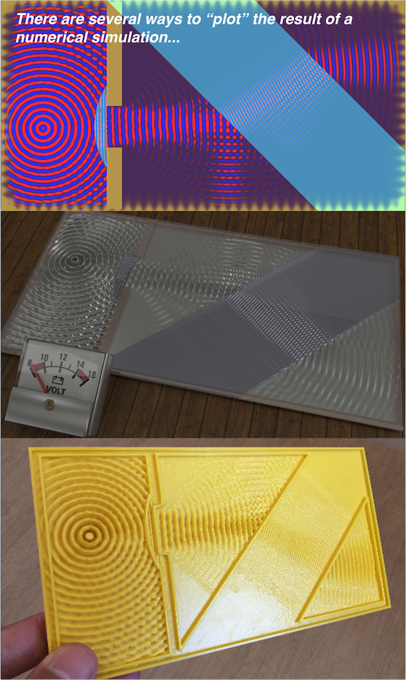

Figure 3: The ways you can visualize the solution to Maxwell’s equation for a boundary condition involving a source, a lens and a tilted glass block.

Conclusions

It is amazing how much knowledge can be extracted from such simple implementation (a loop that calls a function with a simple update rule). The heart of the FD-TD algorithm does not involve while loops or if statements. There is no complex data structures, no weird algorithms and crazy advanced math calculation in the code. Just something like $E[n+1] = E[n] + …$… In the end, the algorithm itself, uses only the 4 mathematical operations. This is the power of Maxwell’s equation. Obviously, we put some considerable effort in the “boundary conditions” by organizing the permittivities, conductivities, etc. But that is a “drawing” effort. The big magic happens because we have such special and carefully crafted relations in the Maxwell’s equations. Nature is REALY amazing!

As I said in the beginning of this post, this is one of my favorite “weekend project”. Not only because I always wanted to simulate Maxwell’s equations themselves. Actually, after I started to play with it, I learned a lot of what is considered very complicated concepts without even notice that I was learning it! One situation that I will aways remember is that, after I arrive in my second post-doc in the Genevra Observatory, I was very scary that I would not understand the optics part of the project. But for my surprise, as I started hearing terms like “diffraction limit”, “point spread function”, “anti-reflex coating”, “sub-aperture” and etc, I began to associate those terms to stuff that I actually saw in my situations, hence knowing exactly what they were!!! That is a feeling that I, as a professor, can’t have enough of.

Thank you for reading this post. I hope you liked reading it as much as I liked writing it! As aways, feel free to comment or share this post as much as you want!