Counting cells

Introduction

In this post I’ll talk about my largest project in terms of time. It started in the middle of year 2000 as my Master thesis subject and ended up extending itself until around mid 2013 (although it remained in hibernation for almost 10 years in between). The project was an “automatic cell counter”. Roughly speaking, it is a computer program that takes an image with two kinds of cells, and tells how many of each kind of cell there is in the image.

At the time, my advisor was professor Adrião Duarte (one of the nicest persons that exists is in this planet). Also, I had no idea about the biology side of things, so I had a lot of help from Dr. Alexandre Sales and Dra. Sarah Jane both from the “Laboratório Médico de Patologia” back in Brazil. They were the best in explaining to me all the medical stuff. Also, they provided a lot of images and testing for the program.

The “journey” was an adventure. From publishing my first international paper, going to Hawaii on my first plane flight, down to asking for funding to buy a microscope in the local financing agency (FAPERN). Although this won’t be a fully technical post, the goal of the post will be to talk about the project itself and things related to it during the .

The problem

The motivation for the project was the need for cell counting in biopsies exams. The process goes more or less like this; When you need a biopsy of some tissue, the pathologist prepares one or more laminas with very very thin sheets of the tissue. The tissue in those laminas are coloured with a special pigment. That pigment has a certain protein designed to attach itself to specifics substances present in the cells that are behaving differently like ongoing division, for instance. The result is that the pigment makes the cells (actually the nucleus) to appear in a different colour depending on the pigment used. Then, we have means to differentiate between the two “kinds” of cells in the lamina.

The next step is to count the cells and compute how many of them is coloured and how many are not. This ratio (percentage of coloured vs non-coluored) will be the result of the biopsy. The problem here is exactly the “counting” procedure. How the heck does one count individual cells? The straight forward way to do that is to put the lamina into the microscope, look into the objective and, patiently and with caution, start counting by eye. Here we see a typical image used in this process. There are hundreds of nucleus (cells) in those kinds images. Even if you capture the image and count them in a screen, the process is tedious! Moreover, the result can’t be based on one single image. Each lamina can produce dozens or hundreds of images that are called fields. To give the result of an exam, several fields have to be counted.
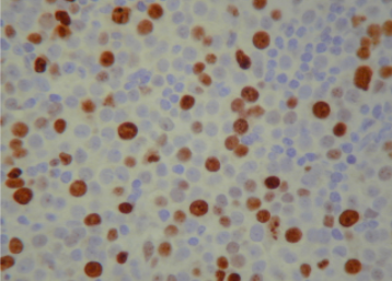
Nowadays, there are machines that do this counting but they are still expensive. At the time I did the project, they were even more expensive and primitive. So, any contribution to this area that would help the pathologist to do this counting more precisely and easily would be very good.

The App

The solution proposed in the project was to make an application (a computer program at the time) that would do this counting automatically. Even at the time, it was relatively easy to put a camera into a microscope. Today it is almost a default 😄. So, the idea was to capture the image from the camera coupled in the microscope, give it as input to the program, and the program would count how many cells are in the image.

Saying it like this, makes it sound simple… But it is not trivial. The cells, as you can see in the previous sample image, are not uniformly coloured, there is a lot of artefacts in the image, the cells are not perfect circles, etc. Hence, I had to device an algorithm to perform this counting.

The algorithm is basically divided in 3 main steps that are very common in image processing solutions;
1 – Pre-Processing
2 – Segmentation
3 – Post-Processing
4 – Counting

Algorithm

The pre-processing stage consisted in applying a colour transform and performing an auto-contrast procedure. The goal was to normalise the images for luminance, contrast, etc. The segmentation step consisted in label each pixel as one of three categories: cell 1, cell 2 or intra-cellar medium (non-cell). The result would be an image where each pixel is either 1, 2 or 3 (or any arbitrary triple of labels). After that comes the most difficult part, which was the post-processing. The segmentation left several cells touching each other or produced a lot of artefacts like tiny regions where there were no cells but was marked as a cell. Hence, the main scientific contribution of the project was to make use of mathematical morphology to process the segmented image and produce an image with only regular pixels in the cells. Finally we have the counting step which resulted in the number of cells labeled as 1 or 2. The technical details of all those steps are in the Masters document or in the papers (see references).

Old windows / web version

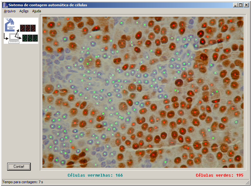
As the final product of the Masters project, I implemented a windows program in C++ Builder with a very simple interface. Basically the user opens an image and press a button to count. That was the program used by Dr. Alexandre in his laboratory to validate the results. I found the old code and made available in GitHub (see references)
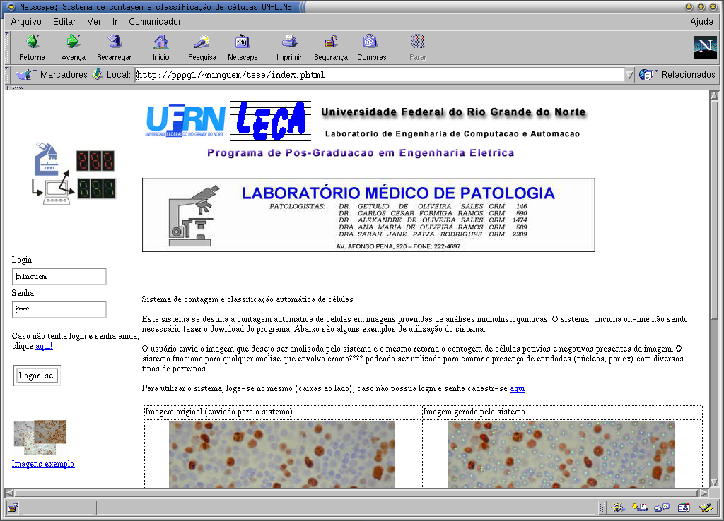
Together with the windows program, I also made an “on-line version” of the application. At the time, an online system that would count cells by uploading an image was a “wonder of technology”😂. Basically it was a web page powered by a PHP script that called a CGI-bin program that did the heavy duty work (implementation of the algorithm) and showed the result. Unfortunately I lost the web page and the CGI code. All I have now is a screenshot that I used in my masters presentation.
iOS

After the Masters defence, for a couple of months I still worked a bit to fix some small stuff and made some small changes here and there. Then, I practically forgot about the project. Dr. Alexandre kept using it for a while but no modifications were made.

Almost 10 years later (around 2012), I was working with iOS development and had the idea of “porting” the program to a mobile platform. Since the iPhone (and iPad) have cameras, maybe we could use to take a picture directly in the objective of the microscope and have the counting right there! So, I did it. I made an app called PathoCounter for iOS that you could take a picture and process the image directly into the device.

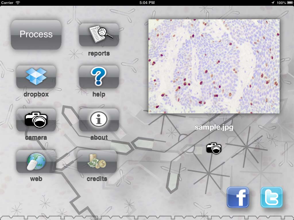
The first version was working only on my phone. Just to be a proof of concept (that worked). Then, I realize that the camera on the phone was not the only advance that those 10 years of moore’s law gave me. There was a godzilion of new technology that I could use in the new version of the project! I could use the touch screen to make the interface easy to operate, and allow the user to give more than just the image to the app. The user could paint areas that he knew there were no cells. We could use more than the camera to take images. We could use Dropbox, web, the gallery of the phone, etc. We could produce a report right on the phone and share with other pathologist. The user could have an account to manage his images. And so on… So I did most of what came to my mind and end up with a kind of “high end” cell counting app and made it available in the Apple store. I even put a small animation of the proteins antigens “fitting” in the cell body 🤣. For my surprise, people started to download it!
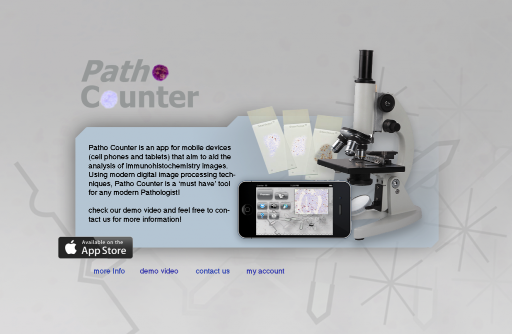
At first I hosted a small web system where the user could login and store images so he could use within the app. I tried to obey some rules for website design but I’m terrible at it. Nevertheless I was willing to “invest my time” to learn how a real software would work. I even learned how to promote a site on facebook and google 😅.
However, I feared that if I had many users the server could not be robust enough, so I tried a crowdfunding campaign at indiegogo.com to buy a good computer to make a private server. For my surprise, some friends baked up the campaign and, in particular, one of my former students Victor Ribas donated $500 dollars! I’m still thankful to him and I was very happy to see such support!! Unfortunately the amount collected wasn’t enough to buy anything different form what I had, so I decided do donate the money to a local Children Hospital that treats children with cancer. Since the goal of the app was to help out with the cancer fight, I figure that the hospital was a good choice for the donation.
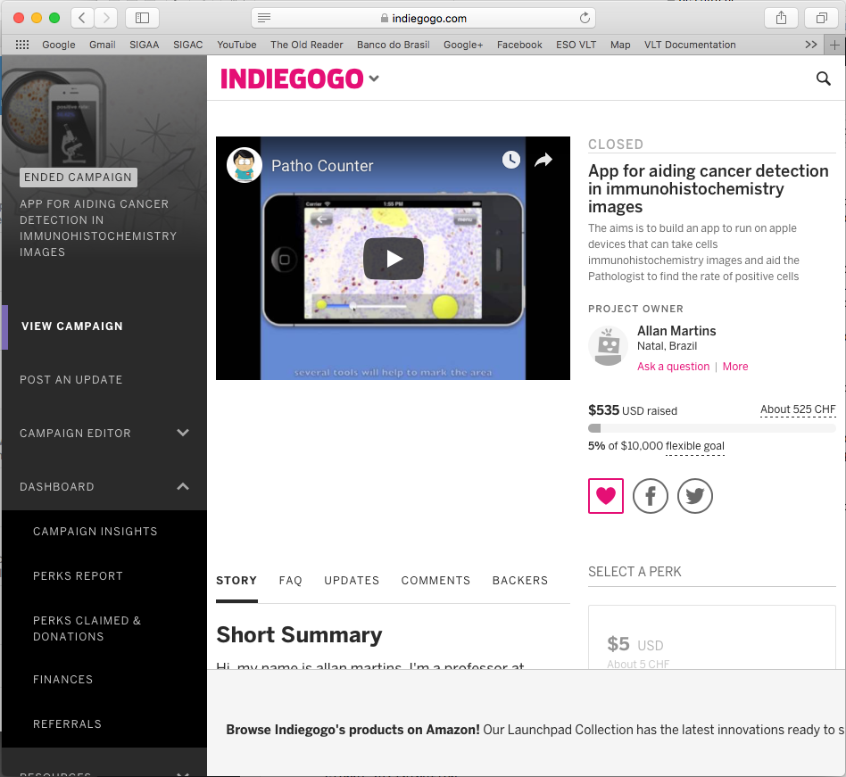
Sadly, this campaign also attracted bad audience. A couple of weeks after the campaign closed and I donated the money, I was accused (formally) of doing unethical fund-gathering for public research. Someone in my department filed a formal accusation against me, and, among some things, told that I was obtaining people’s money from unsuccessful crowdfunding campaigns. That hurts a lot. Even though it was easy to write a defence because I didn’t even kept the money, I had to call the Hospital I did the donation and ask for a “receipt” to attach as a proof in the process. They had offered a receipt at the time I made the donation, but I never imagined that two weeks later I would go though this kind of situation. So, I told them that wasn’t necessary because I was not a legal person or company, and I didn’t want to bother them with the bureaucracy.

Despite this bad pebble in the path, everything that followed was great! I had more the 1000 downloads all around the world. That alone was enough to make me very happy. I also decided to keep my small server running. Some people even got to use the server, although just a handful. Another cool thing that happened was that I was contacted by two pathologists outside Brazil; one from Italy and another from United States. The app was free to download and the user had 10 free exams as a demo. After that the user could buy credits, which nobody did 😂 (I guess because you just could reinstall the app to get the free exams again 😂). I knew about that “bug”, but I was so happy to see that people were actually using the app that I didn’t bother (although Dr. Alexandre told me that I was a “dummy” to not properly monetise the app 🤣).

The app was doing so much more than I expected that I even did some videos explaining the usage. Moreover, I had about 2 or 3 updates. They added some small new features, fixed bugs, etc. In other words, I felt like I was developing something meaningful, and people were using it!

Results

As I said, the main result to me was the usage. To know that people were actually using my app felt great. Actually, the girl from United States that contacted me said that they were using it in dog exams! I didn’t even knew that they did biopsy in animals 😅.

Analytics

At the time I was into the iOS programming “vibe” I use to put a small module in all my apps to gather anonymous analytics data (statistics of usage). One of the data I gathered, when the user permitted of course, was the location were the app was being used. Basically every time you used the software, the app sent the location (without any information or identification of the user whatsoever) and I stored that location. After one or two year of usage, this was the result (see figure).
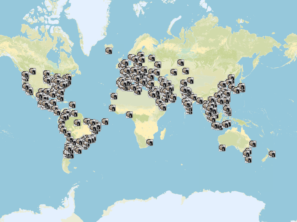
Each icon is a location where the app was used and the user agreed in sharing the location. The image speaks for itself. Basically all the continents were using the app. That is the magic of online stores nowadays. Anybody can have your app being used by, easily, thousands of people! I’m very glad that I lived this experience of software development 😃.

Media

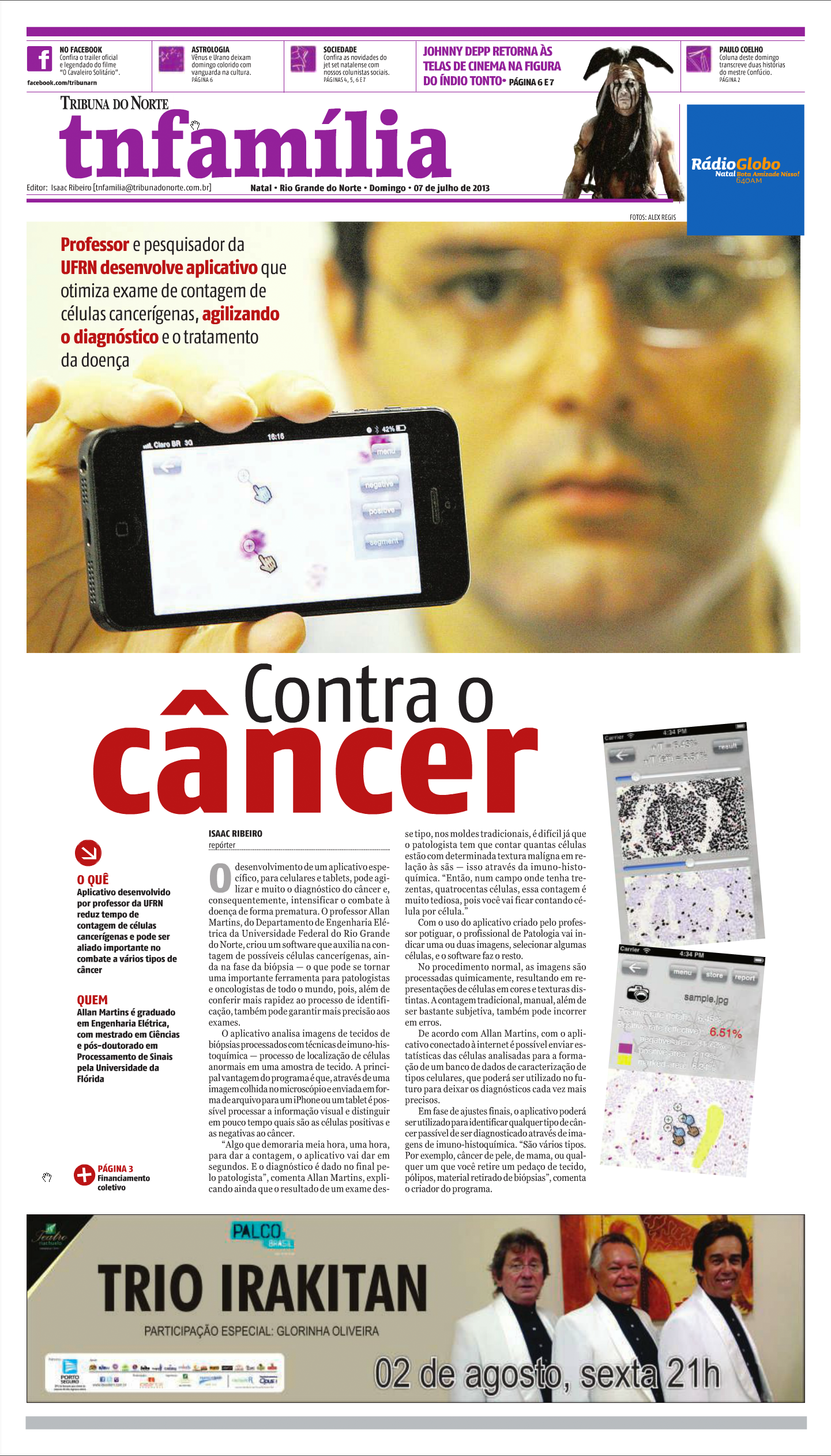
Somehow the app even got the media’s attention. A big local newspaper and one of the public access TV channels here in my city, contacted me. They asked if they could write an article about the app and interview me about it 🤣😂. I told them that I would look bad in front of the camera but I would be very happy to talk about the app. Here goes the first page of the newspaper article in the “Tribuna do Norte” newspaper and the videos of the interviews (the TV Tribuna and TV Universitária UFRN).
Conclusion

I don’t know for sure if this app helped somebody to diagnose an early cancer or helped some doctor to prescribe a more precise dosage of some medicine. However, it shows that everyone has the potential to do something useful. Technology is allowing advances that we could never imagine (even 10 years before when I started my masters). The differences in technology from 2002 to 2012 are astonishing! From a Windows program, going through an online web app, to a worldwide distributed mobile app, software development did certainly changed a lot!

As always, thank you for reading this post. Please, feel free to share it if you like. See you in the next post!

References

Wikipedia – Immunohistochemistry

C++ Builder source

Sistema de Contagem e Classificação de Células Utilizando Redes Neurais e Morfologia Matemática – Tese de Mestrado

MARTINS, A. M.; DÓRIA NETO, Adrião Duarte ; BRITO JUNIOR, A. M. ; SALES, A. ; JANE, S. Inteligent Algorithm to Couting and Classification of Cells. In: ESEM, 2001, Belfast. Proceedings of Sixth Biennial Conference of the European Sorciety for Engineer and Medicine, 2001.

MARTINS, A. M.; DÓRIA NETO, Adrião Duarte ; BRITO JUNIOR, A. M. ; SALES, A. ; JANE, S. Texture Based Segmentation of Cell Images Using Neural Networks and Mathematical Morphology. In: IJCNN, 2001, Washington. Proceedings of IJCNN2001, 2001.

MARTINS, A. M.; DÓRIA NETO, Adrião Duarte ; BRITO JUNIOR, A. M. ; FILHO, W. A. A new method for multi-texture segmentation using neural networks. In: IJCNN, 2002, Honolulu. Proceedings of IJCNN2002, 2002.

3+

Wavefront sensing

Introduction

Wavefront sensing is the act of sensing a wave front. As useless as this sentence gets, it is true and we perform this action with a wavefronts sensor… But if you bare with me, I promise that its going to be one of the coolest mix of science and technology that you will hear about! Actually, I promise that it would be even poetic, since that, in this post, you will learn why the stars twinkle in the sky!

Just a little disclaim before I start: Im not an optical engineer and I understand very little about the subject. This post is just myself sharing my enthusiasm about this amazing subject.

Well, first of all, the word sensing just mean “measure”. Hence, wavefront sensing is the act of measure a wave front with a wavefront sensor. To understand what a wavefront measurement is, let me explain what a wavefront is and why one would want to measure it. It has to do with light. In a way, wavefront measurement is the closest we can get from measuring the “shape” of a light wave. The first time I came across this concept (here in the Geneva observatory) I asked myself: “What does that mean? Doesn’t light has the form of its source??”. I guess thats a fair question. In the technical use of the term measurement, we consider here that we want to measure the “shape” of the wave front that was originated in a point source of light very far away. You may say: “But thats just a plain wave!” and you would be right if we were in a complete homogeneous environment. If that were the case, we would have nothing to measure %-). So, what happens when we are in a non-homogenous medium? The answer is: The wavefront gets distorted, and we got to measure how distorted it is! When light propagates as a plain wave and it passes through an non-homogeneous medium, part of its wavefront slows down and others don’t. That creates a “shape” in the phase of the wavefront. Because of the difference in the index of refraction of the medium, in some locations, the oscillation of the electromagnetic arrives a bit earlier and some other it arrives a bit later. This creates a diferente in phase at each point in space. The following animation tries to convey this idea.

Figure 1: Wavefront distorted by a medium

As we see in the animation, the wavefront is plain before reaching the non-homogeneous medium (middle part). As it passes through the medium, it exits with a distorted wavefront. Since the wavefront is always traveling in a certain direction, we are only interested in measure it in a plane (in the case of the animation, a line) perpendicular to its direction of propagation.

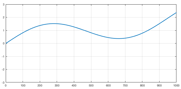
In the animation above, a measurement at the left side would result in a constant value since, for all “y” values of the figure, the wave arrives at the same time. If we measure at the left side we get something like this

Figure 2: Wavefront measurement for the medium showed in Figure 1

Of course that, in a real wavefront, the measurement would be 2D (so the plot would be a surface plot).

An obvious question at this point is: Why someone would want to measure a wavefront? There is a lot os applications in optics that requires the measurement of a wavefront. For instance, lens manufacturer would like to know if the shape of the lenses they manufactured is within a certain specification. So they shoot a plane wavefront through the lens of the glass and measure the deformation in the wavefront causes by the lens. By doing that, they measure the lens properties like astigmatism, coma and etc. Actually, did you ever asked yourself where those names (defocus, astigmatism, coma) came from? Nevertheless, one of the the most direct use of this wavefront measuring is in astronomy! Astronomers like to look at the stars. But the stars are very far away and, for us, they are an almost perfect point source of light. That means that we should receive a plain wave here right? Well if we did we have nothing to breath! Yes, the atmosphere is the worst enemy of the astronomers (thats why they spend millions and millions to put a telescope in orbit). When the light of the star or any object passes through the atmosphere, it gets distorted. Its wavefront make the objet’s image swirl and stretch randomly. Worst then that, the atmosphere is always changing its density due to things like wind, clouds and difference in temperatures. So, the wavefront follows this zigzags and THAT is why the stars twinkle in the sky! (I promise didn’t I? 😃) So, the astronomers build sophisticated mechanisms using adaptive optics to compensate for this twinkling and that involves, first of all, to measure the distortion of the wavefront.

Wavefront measurement

So, how the heck do we measure this wavefront? We could try to put small light sensors in an array and “sense” the electromagnetic waves that arrives at them… But light is pretty fast. It would be very very difficult to measure the time difference between the rival of the light in one sensor compared to the other (the animation in figure 1 is like a SUPER MEGA slow motion version of the reality). So, we have to be clever and appeal to the “jump of the cat” (expression we use in Brazil to mean a very smart move to solve a problem).

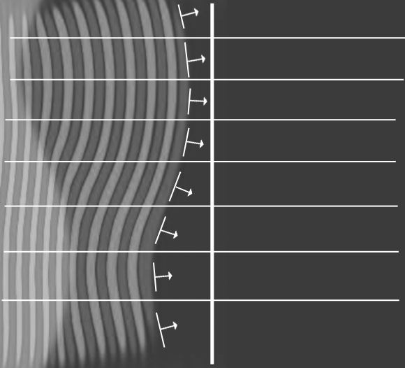
In fact, the solution is very clever! Although there are different kinds of wavefront sensors, the one I will explain here is called Shack–Hartmann wavefront sensor. The ideia is amazingly simple. Instead of measuring directly the phase of the wave (that would be difficult because light travels too fast) we could measure the “inclination” or the local direction of propagation of the wavefront. Now, instead of an array of light sensors that would try to measure the arrival time, we make an array of sensors that measure the local direction of the wavefront. With this information it is possible to recover the phase of the wavefront, but that is a technical detail. So, in summary, we only need to measure the angles of arrival of the wavefront. Figure 3 tries to exemplify that I mean:

Figure 3: Exemple of measurement of direction of arrival, instead of time of arrival.

Each horizontal division in the figure is a “sub-aperture” where we measure the inclination of the wavefront. Basically we measure the angle of arrival, instead of the time of arrival (or phase of arrival). If we do those sub-apertures small enough, we can reconstruct a good picture of the wavefront. Remember that for real wavefronts we have a plane, so we should measure TWO angles of arrival for each sub-aperture (the angle in x and the angle in y, considering that z is the direction of propagation).

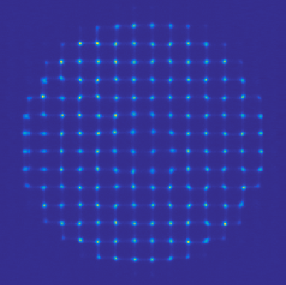
At this point you might be thinking: “Wait… you just exchanged 6 for 12/2! How the heck do we measure this angle of arrival? It seems that this is far more difficult then to measure the phase itself!”. Now its time to get clever! The idea is to put a small camera in each sub aperture. Each tiny camera will be equipped with a tiny little lens to focus the portion of the wavefront to a certain pixel of this tiny camera! Doing that, at each camera, depending on the angle of arrival, the lens will focus the locally plain wave to a certain region of the camera dependent on the direction its traveling. That will make each camera see a small region with bright pixels. If we measure where those pixels are in relation to the center of the tiny camera, we have the angle of arrival!!! You might be thinking that its crazy to manufacture small cameras and small lenses in a reasonable packing. Actually, what happens is that we just have the tiny lenses in front of a big CCD. And it turns out that we don’t need hight resolution cameras in each sub-aperture. A typical wavefront sensor has 32×32 sub apertures, each one with a 16×16 grid os pixels. That is enough to give a very good estimation of the wavefront. Figure 4 shows a real image of a wavefront sensor.

Figure 4: Sample image from a real wavefront sensor

Simulations!

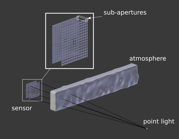
The principle is so simple that we can simulate it in several different ways. The first one is using the “light ray approach” for optics. This principle is the one we learn in college. Its the famous one that they put a stick figure on one side of a lens or a mirror and them draw some lines representing the light path. The wavefront sensor would be a bit more complex to draw, so we use the computer. Basically what I did was to make a simple blender file that contains a light source, something for the light to pass through (atmosphere) and the sensor itself. The sensor is just an 2D array of small lenses (each one made up by two spheres intersected) and a set of planes behind each lens to receive the light. We then set up a camera between the lenses and the planes to be able to render the array of planes, as they would be the CCD detectors of the wavefront sensor. Now we have to set the material for each object. The “detectors” must be something opaque so we could see the light focusing on it. The atmosphere have to be some kind of glass (with a relatively low index of refraction). The lenses also have glass as its material, but their index of refraction must be carefully adjusted so the focus of each one can be exactly on the detectors plane. Thats pretty much it (see figure 5).

Figure 5: Setup for simulating a wavefront sensor in blender

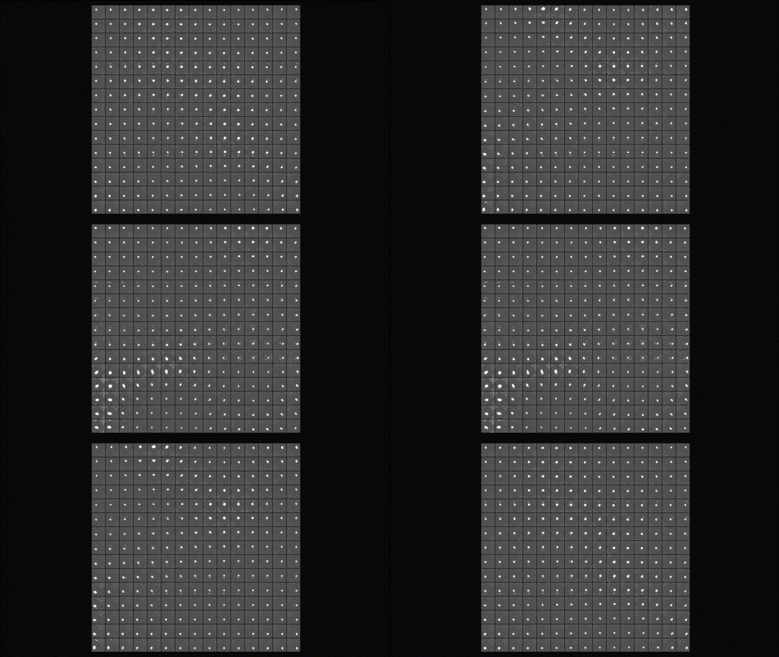
To simulate the action, we move the “atmosphere” object back and forth and render each step. As light passes through the object, it diffracts it. That changes the direction of the light rays and simulates the wavefront being deformed. The result is showed in figure 6.

Figure 6: Render of the image on the wavefront sensor as we move the atmosphere simulating the real time reformation of the wavefront.

Another way of simulating the wavefront sensor is to simulate the light wave itself passing through different mediums, including the leses themselves and driving at some absorbing material (to emulate the detectors). That sounds kind of hardcore simulation stuff, and it kind of is. But, as I said in the “about” of this blog, I’m curious and hyperactive, so here we go: Maxwells equations simulation of a 1D wavefront sensor. To do that simulation, I used a code that I did a couple of yeas back. I’ll make a post about it some day. It is an implementation of a FD-TD (Finite Diferences in the Time Domain) method. This is a numerical method to solve partial differential equations. Basically, you set up your environment as a 2D grid with sources of electromagnetic field, material of each element on the grid and etc. Then, you run the interactive method to see the electromagnetic fields propagating. Anyway, I put some layers of conductive material to contain the wave is some points and to emulate the detector. Then I added a layer with small lenses with the right refraction index to emulate the sub-apartures. Finally, I put a monochromatic sinusoidal source in one place and pressed run. Voilá! You can see the result in the video bellow. The video contains the explanation of each element and, as you can see, the idea of a wavefront sensor is so brilliantly simple that we can simulate it at the Maxwells equation level!

DIY (physical) experiment

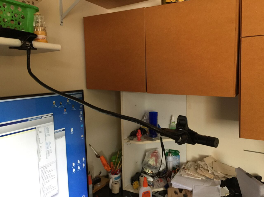
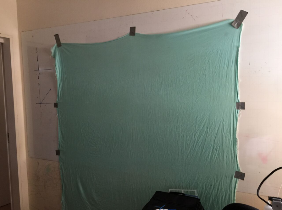
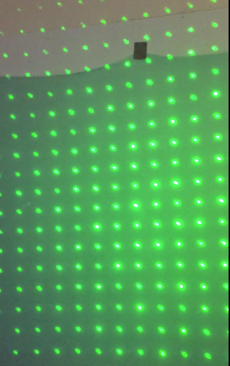
To finish this post, let me show you that you can even build your own wavefront sensor “mockup” at home! What I did in this experiment was to build a physical version of the Shack–Hartmann principle. The idea is to use a “blank wall” as detector and a webcam to record the light that arrives at the wall. This way I can simulate a giant set of detectors. Now the difficult part: the sub-aperure lenses… For this one, I had to make the cat jump. Instead of an array of hundreds of lenses in front of the “detector wall”, I uses a toy laser that comes with those diffraction crystals that projects “little star-like patterns” (see figure 7).

Figure 7: 1 – Toy laser (black stick) held in place. 2 – green “blank wall”. 3 – Diffraction pattern that generates a regular set of little dots.

With this setup, it was time to do some coding. Basically I did some Matlab functions to capture the webcam image of the wall with the dots. On those functions I setup some calibration computations to compensate for the shape and place of the dots on the wall (see video bellow). That calibration will tell me where the “neutral” atmosphere will project the points (centers of the sub apertures). Them, for each frame, I capture and process the image from the webcam. For each image, I compute the position of the processed centers with respect to the calibrated ones. With this procedure, I have, for each dot, a vector that points form the center to where it is. That is exactly the wavefront direction that the toy laser is emulating!

After that, it was a matter of having fun with the setup. I put all kinds of transparent materials in front of the laser and saw the “vector field” of the wavefront directions on screen. I even put my glasses and were able to see the same pattern the optical engineering saw when they were manufacturing the lenses! With a bit of effort I think I could even MEASURE (poorly of course) the level of astigmatism of my glasses!

The code is available in GitHub[2] but basically the loop consists in process each frame and show the vector field of the wavefront.

while 1
    newIcap = cam.snapshot();
    newI = newIcap(:,:,2);
    newBW = segment(newI, th);
    
    [newCx, newCy] = processImage(newBW, M, R);
    
    z = sqrt((calibratedCy-newCy).^2 + (calibratedCx-newCx).^2);
    zz = imresize(z,[480, 640]);
    
    figure(1);
    cla();
    hold('on');
    imagesc(zz(end:-1:1,:), 'alphadata',0.2)
    quiver(calibratedCy, calibratedCx, calibratedCy-newCy, calibratedCx-newCx,'linewidth',2);
    
    axis([1 640 1 480])
    
    drawnow()
end
  Bellow you can watch the vídeo of the whole fun!

Conclusions

DIY projects are awesome for understanding theoretical concepts. In this case, the mix of simulation and practical implementation made very easy to understand how the device works. The use of the diffraction crystal in toy lasers is thought to be original, but I didn’t research a lot. If you know any experiment that uses this same principle, please let me know in the comments!

Again, thank you for reading until here! Feel free to comment o share this post. If you are an optical engineer, please correct me at any mistake I might have made on this post. It does not intend to teach about optics, but rather to share my passion for this subject that I know so little!

Thank you for reading this post. I hope you liked it and, as always, feel free to comment, give me feedback, or share if you want! See you in the next post!

References

[1] – Shack–Hartmann wavefront sensor

[2] – Matlab code

2+