Introduction
Since I was a kid, I always loved toys with “moving parts”. In particular, I was always fascinated with the transmission of the movement between two parts of a toy. So, whenever a toy had “gears” in it, for me, it looked “sophisticated”. This fascination never ended and a couple of year ago when I bought my 3D printer, I wanted to build my own “sophisticated” moving parts and decided to print some gears.I didn’t want to just download gears from thingverse.com and simple print them. I wanted to be able to design my own gears in the size I want with the specifications I needed. Well… I’d never thought a would have so much fun…
So, in this post I will talk briefly about this little weekend project of mine: Understanding a tiny bit about gears!
The beautiful math behind it
At first I thought that the only math that I needed was the following \[ \frac{{{\omega _1}}}{{{\varpi _2}}} = \frac{{{R_2}}}{{{R_1}}} \] In another words, the ratio of the angular speeds is proportional to the ratio of the radius of the gears. Everyone know that, right? If you have a large gear and a small one, you have to rotate the small one a lot to rotate the big one a little. So, to make a gear pair that doubles the speed I just had to make one with, say, 6cm of diameter and the other with 3cm. Ha… but how many teeth? What should be their shape? Little squares? Little triangles? These questions started to pop and I was getting more and more curious.At first I thought I use a simple shape for the teeth. I would not put too many teeth because they could wear out with use. Also, not too few because they had to be big and I might end up with too much slack. Gee, the thing started to get complicated. So, I decided to research a bit. For my surprise I found out that the subject “gears” is a whole area in the field of Mechanical Engineering. First thing I notice is that most of the gears have a funny rounded shape for the teeth. Also, they had some crops and hollow spaces in the teeth that vary from gear to gear. Clearly those were there for a reason.
Those “structures” are parameters of the gear. Depending on the use, material or environment, they can be chosen at design time to optimise the gear function. However, practically all gears have one thing in common : The contact of the gear teeth must be optimum! It must be such that during rotation, the working gear tooth (the one that is being rotated) must “push” the other gear tooth in such a way that the contact is always perpendicular to the movement as if we had a linear or straight object pushing another in a straight movement. Moreover, the movement must be such that when one tooth leaves the contact region, another tooth must take over, so the movement is continuous (see figure).
Figure 1: Movement being transmitted from one tooth to another. The contact and the force is always perpendicular and is continuously transmitted as the gear rotates. (source: Wikipedia. See references)
This last requirement can mathematically be archived by a curve called “Involute”. Involute is a curve that is made when you take a closed curve (a circle for example) and start to “peel of” it’s perimeter. The “end” of the peeling is the points in the involute (see figure).
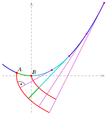
Figure 2: Two involute curves (red). Depending on the starting point, we have different curves. (source: Wikipedia. See references)
So, the shape of the teeth of the gears are involutes of the original gear shape. Actually not all gears are like that. The gears that are, are called “Involute Gears”. Moreover, gears do not need to be circular. If you have a gear with another shape, you just need to make its teeth curved as the involute of the shape of the gear.The question now is: How to find the involute of a certain shape?
Following the “peeling” definition of the involute, it is not super hard to realise that the relationship between the involute and its generating curve is that, at each point in the involute curve, a line perpendicular to it will be tangent to the original curve. With that, we have the following relation: \[ \begin{array}{*{20}{l}} {\dot X(t)\sqrt {{{\dot x}^2}(t) + {{\dot y}^2}(t)} = \dot y(t)\sqrt {{{(x(t) – X(t))}^2} + {{(y(t) – Y(t))}^2}} } \\ {\dot Y(t)\sqrt {{{\dot x}^2}(t) + {{\dot y}^2}(t)} = – \dot x(t)\sqrt {{{(x(t) – X(t))}^2} + {{(y(t) – Y(t))}^2}} } \end{array} \] Which is a weird looking pair of differential equations! There, \((X(t), Y(t))\) is the parametric curve for the involute and \((x(t), y(t))\) is the parametric curve for the original curve.
Some curves do simplify this a lot. For instance, for a circle (that will generate a normal gear) the solution is pretty simple: \[ \begin{array}{l} X(t) = r\left( {\cos (t) + t\sin (t)} \right)\\ Y(t) = r\left( {\sin (t) – t\cos (t)} \right) \end{array} \]
Matlab fun
So, how do we go from the equation of one involute to the drawing of a set of teeth?To test the concept, first I implemented some Matlab scripts to draw and animate some gears. In my implementation I used a circular normal gear, so the original curve is a circle. Nevertheless, I implemented the differential equation solver using Euler’s method so I could make weird shape gears (in a future project). The general idea is to draw one pieces of involutes starting at each tooth and going to half of the tooth. Then, draw the other half starting from the end of the tooth until the end of it. The “algorithm” to draw a set of involute teeth is the following
- Define the radius and number of teeth
- define \(t = \theta\) and \(dt = d\theta\) (equal to some small number that will be the integration step)
- Repeat for each n from 0 to N-1 teeth:
- Start with \( \theta = n\frac{2\,\pi}{N}\)
- update the involute curve (Euler’s method)
\(X(\theta) = X(\theta) + {\dot X(\theta)}\,d\theta \)
\(Y(\theta) = Y(\theta) + {\dot Y(\theta)}\,d\theta \)
until half of the current tooth - Update the angle in the clockwise duration \( \theta = \theta + d\theta\)
- Start with \( \theta = (n+1)\frac{2\,\pi}{N}\)
- update the involute curve
\(X(\theta) = X(\theta) + {\dot X(\theta)}\,d\theta \)
\(Y(\theta) = Y(\theta) + {\dot Y(\theta)}\,d\theta \)
until half of the current tooth - Update the angle in the anti-clockwise duration \( \theta = \theta – d\theta\)
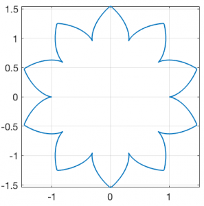
Figure 3: Example of a gear with all auxiliary parameters equal to zero
When you use the technical parameters for a gear, it starts to shape familiar. The main parameters are called “addendum”, “deddendum” and “slack”. Each one control some aspect of the mechanical characteristics of the gear like flexibility of the teeth, depth of the teeth, etc. The next figure illustrates those parameters.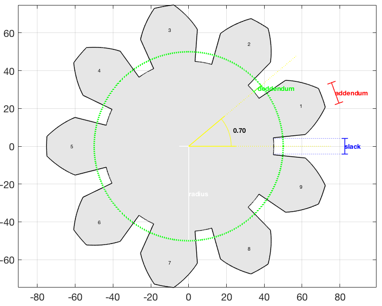
Figure 4: Parameters of a gear
The next step was to position a pair of gears next to each other. First, we choose the parameters for the first gear (addendum, radius, number of teeth, etc). For the second one, we choose everything but the number of teeth. That must be computed form the ratio of the radius.For the positioning, we would put the first gear at the position \((0.0, 0.0)\) and the second one at some position \((x_0,0.0)\). Unfortunately the value of \(x_0\) is not simply \(r_1 + r_2\) (sum of the radius) because the involutes for the teeth must touch at a single point. To solve this, I used a brute force approach. I’m sure that there is a more direct method, but I was eager to draw the pair %-). Basically, I computed the curve for the right gear first tooth and the left gear first tooth (rotated \(2\pi/N\) so they can match when in the right position). Initially I positioned the second one at \(r_1 + r_2\) and displaced bit by bit until they touched only in only one place. In practice I had to deal with a finite number of points for each curve, so I had to set a threshold to consider that the two curves are “touching” each other.
With the gears correctly positioned it was time to make a 3D version of them. That was easy because I had the positions for each point in the gears. So, for each pair of points in each gear I “extruded” a rectangular patch by \(h_0\) in the z direction. Then I made a patch with the gear points and copied another one at \(z = h_0\). Voilà! Two gears that match perfectly!
The obvious next step was to animate them 😃! That is really simple because we just need to rotate the first by a small amount, rotate the second by this amount times the radius ration and keep doing that while drawing the gear over and over. The result is a very satisfying gear pair rotating!
Figure 5: Animations of two gear sets with different parameters.
Blender fun
Now that I got used to the “science”, I was ready to 3D print some gears. For that, I had to transfer the design to Blender, which is the best 3D software in the planet. The problem is that it would be a pain in the neck to design the gear in Matlab, export to something like stl format, test it in Blender and, if it’s not quite what I wanted, repeat the process, etc. So, I decided to make a plugin out of the algorithms. Basically I just implemented all the Matlab stuff in python, following the protocol for a Blender plugin. The result was a plugin that adds a “gear pair” object. The plugin adds a flat gear pair. In general we must extrude the shapes to whatever depth we need in the project. But the good thing is that we can tune the parameters and see the results on the fly (see bellow).Figure 5: Blender plugin
With the gears in blender, the sky is the limit. So, it was time to 3D print some. I did a lot of tests and printed a lot of gears. My favourite so far is the “do nothing machine” gear set (see video) it is just a bunch of gears with different sizes that rotates together. My little daughter loves to keep rotating them 😂!Figure 6: Test with small gears
Figure 7: Do nothing machine with gears
Conclusions
As always, the goal of my posts is to share my enthusiasm. Who would have thought that a simple thing like a gear would involve hard to solve differential equations and such beautiful science with it!Thanks for reading! See you in the next post!
References
[1] – Wikipedia – Involute Gears[2] – Wikipedia – Involute Curve
[3] – GitHUB – gears
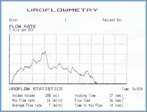 Figure 1 : Sample of a Uroflowmetry result[3]
Then, he prescribe a very common medicine to improve the results and told me that I would repeat the exam a couple of days later. After about 4 or 5 days I returned to the second exam. I repeated the whole process and peed on the USD $10,000.00 toilet. This time I did’t feel I did my “average” performance. I guess some times you are nervous, stressed or just not concentrated enough. So, as expected, the results were not ultra mega perfect. Long story short, the doctor acknowledge the result of the exam and conducted the rest of the visit (I’m fine, if you are wondering heheheh).
Figure 1 : Sample of a Uroflowmetry result[3]
Then, he prescribe a very common medicine to improve the results and told me that I would repeat the exam a couple of days later. After about 4 or 5 days I returned to the second exam. I repeated the whole process and peed on the USD $10,000.00 toilet. This time I did’t feel I did my “average” performance. I guess some times you are nervous, stressed or just not concentrated enough. So, as expected, the results were not ultra mega perfect. Long story short, the doctor acknowledge the result of the exam and conducted the rest of the visit (I’m fine, if you are wondering heheheh).
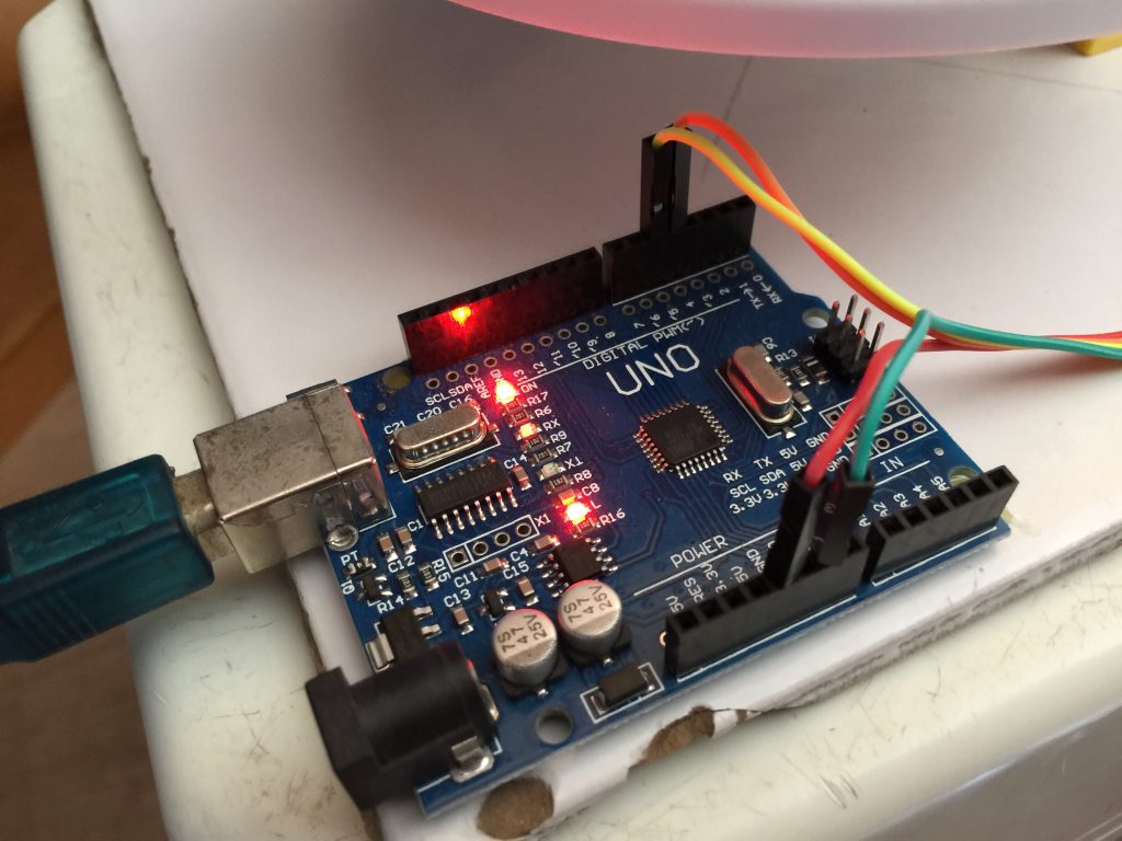 Figure 2 : Arduino board
First I had to make the digital scale, so I used a load cell that had the right range for this project. The weight of the urine would range from 0 to 300~500mg more or less, so I acquire a 2Kg range load cell (Figure 3 and 4). I disassemble an old kitchen scale to use the “plate” that had the right space to hold the load cell and 3D printed a support in a heavy base to avoid errors in the measurements due to the flexing of the base. For that, I used a heavy ceramic tile that worked very well. The cell “driver” was an Arduino library called HX711. There is a cool youtube tutorial showing how to use this library [1].
Figure 2 : Arduino board
First I had to make the digital scale, so I used a load cell that had the right range for this project. The weight of the urine would range from 0 to 300~500mg more or less, so I acquire a 2Kg range load cell (Figure 3 and 4). I disassemble an old kitchen scale to use the “plate” that had the right space to hold the load cell and 3D printed a support in a heavy base to avoid errors in the measurements due to the flexing of the base. For that, I used a heavy ceramic tile that worked very well. The cell “driver” was an Arduino library called HX711. There is a cool youtube tutorial showing how to use this library [1].
 Figure 3 : Detail of the load cell used to make the digital scale.
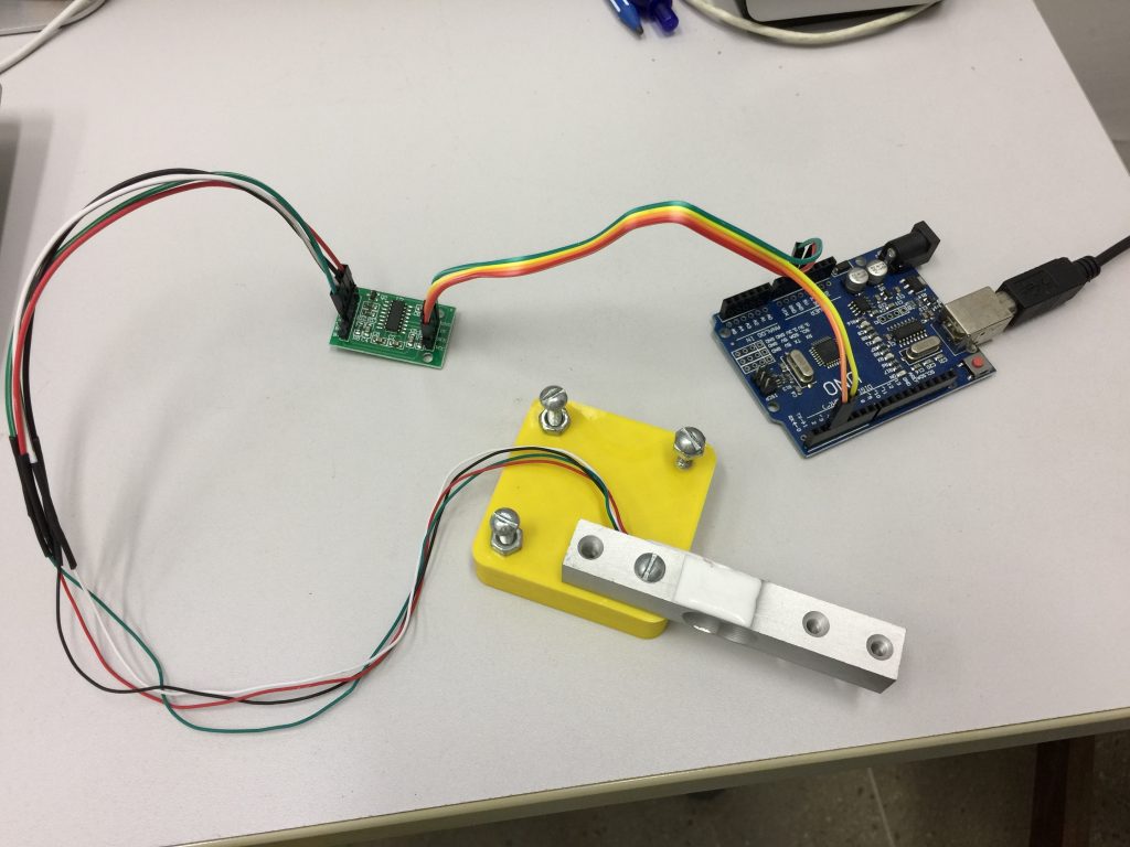 Figure 4 : Loadcell connected to the driver HX711
The next problem was how to connect to the computer!!! This is not a regular project that you can assemble everything on your office and do tests. Remember that I had do pee on the hardware! I also didn’t want to bring a notebook to the bathroom every time I want to use it! the solution was to use a wifi module and communicate wirelessly. Figure 5 shows the module I used. Its an ESP8266. Now I could bring my prototype to the bathroom and pee on it while the data would be sent to the computer safely.
Figure 4 : Loadcell connected to the driver HX711
The next problem was how to connect to the computer!!! This is not a regular project that you can assemble everything on your office and do tests. Remember that I had do pee on the hardware! I also didn’t want to bring a notebook to the bathroom every time I want to use it! the solution was to use a wifi module and communicate wirelessly. Figure 5 shows the module I used. Its an ESP8266. Now I could bring my prototype to the bathroom and pee on it while the data would be sent to the computer safely.
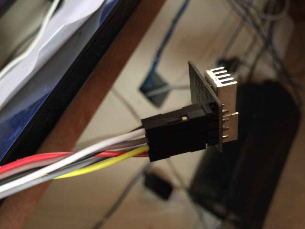 Figure 5 : ESP8266 connection to the Arduino board.
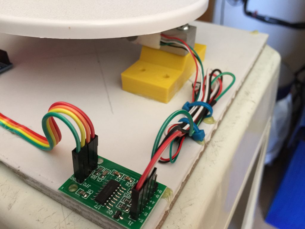
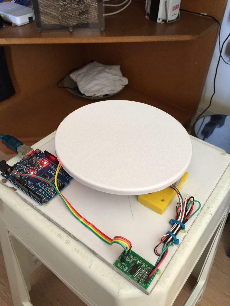
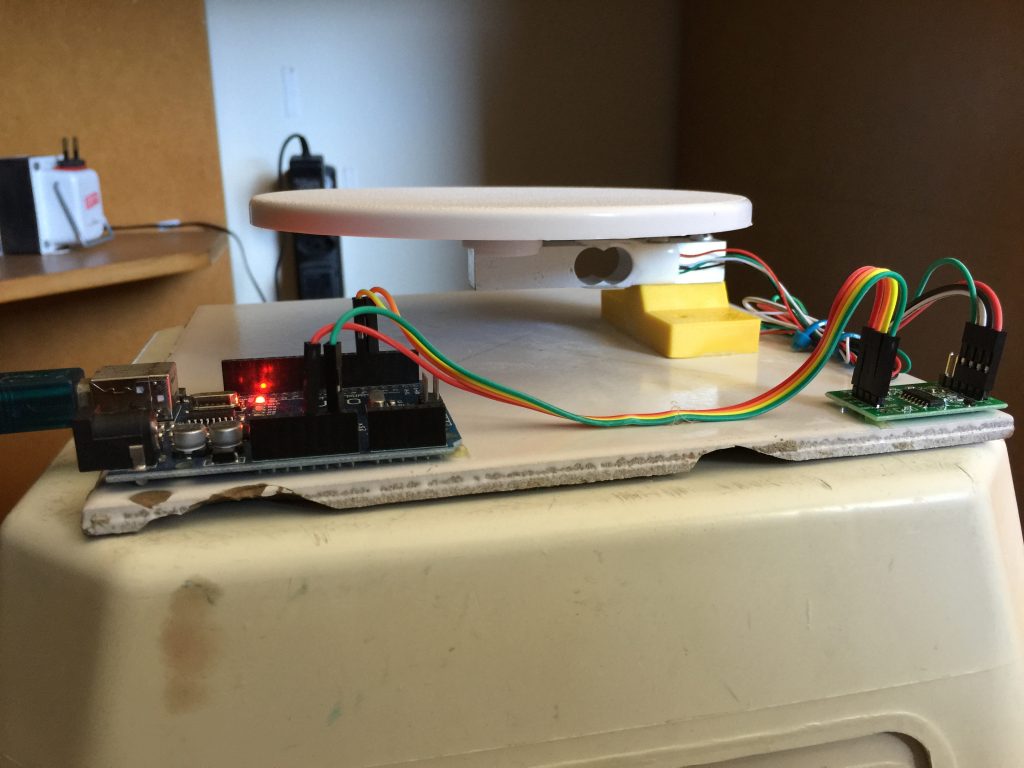
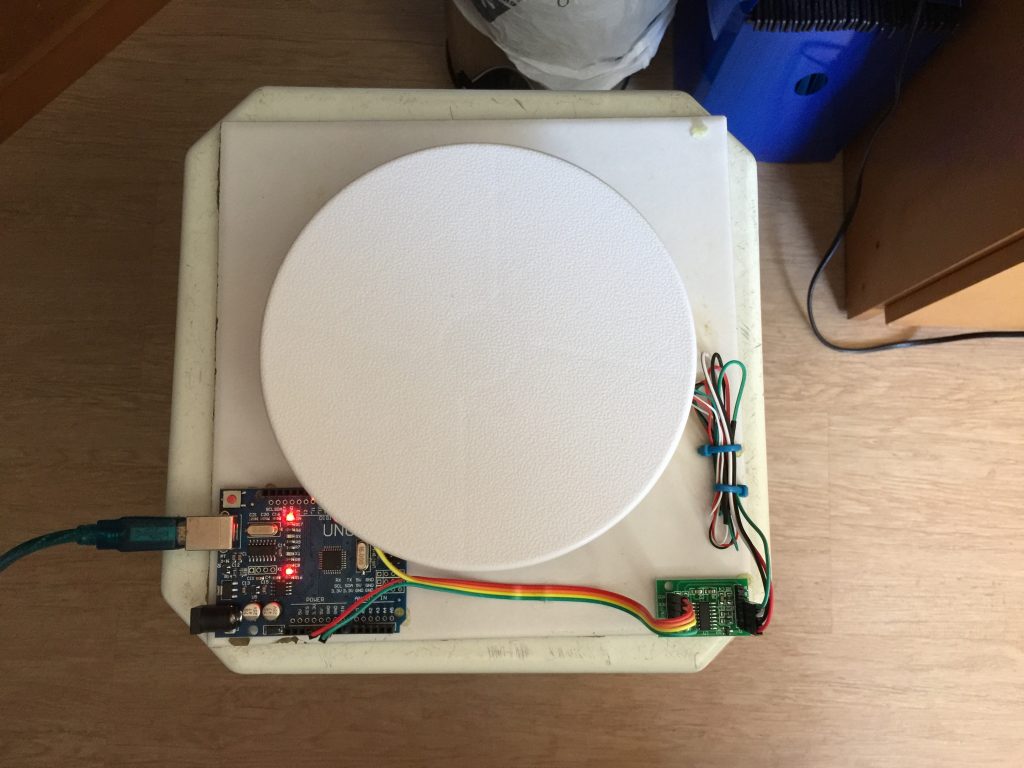 Figure 6 : More pictures of the prototype
Once built, I had to calibrate it very precisely. I did some tests to measure the sensibility of the scale. I used an old lock and a small ball bearing to calibrate the scale. I went to the laboratory of Metrology at my university and a very nice technician in the lab (I’m so sorry I forgot his name, but he as very very kind) measures the weights of the lock and the ball bearing in a precision scale. Then I started to do some tests (see video bellow)
The last thing to make the prototype 100% finished was to have a funnel that had the right size. So I 3D printed a custom size funnel I could use (figure 7).
Figure 6 : More pictures of the prototype
Once built, I had to calibrate it very precisely. I did some tests to measure the sensibility of the scale. I used an old lock and a small ball bearing to calibrate the scale. I went to the laboratory of Metrology at my university and a very nice technician in the lab (I’m so sorry I forgot his name, but he as very very kind) measures the weights of the lock and the ball bearing in a precision scale. Then I started to do some tests (see video bellow)
The last thing to make the prototype 100% finished was to have a funnel that had the right size. So I 3D printed a custom size funnel I could use (figure 7).
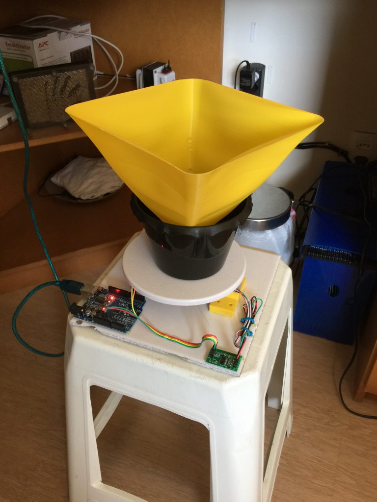
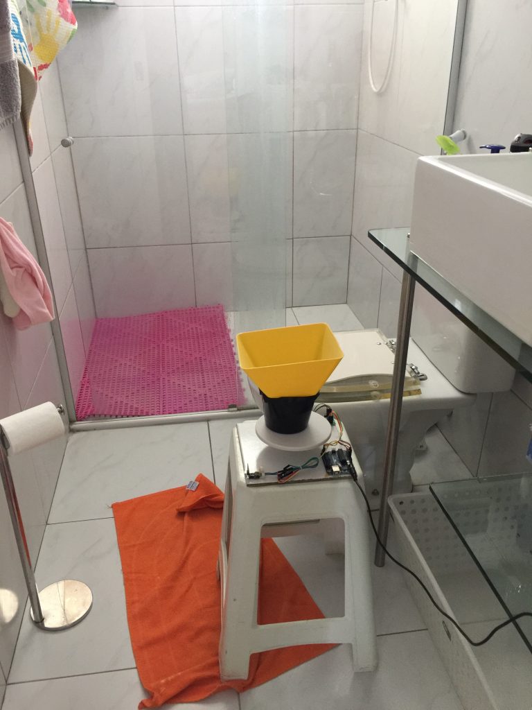 Figure 7: Final prototype ready to use
Once calibrated and ready to measure weights in real time, It was time to code the flow calculation. At first, this is a straight forward task, you just differentiate the measurements in time. Something like
$$
\begin{equation}
f[n] = \frac{{w[n – 1] – w[n]}}{{\rho \Delta t}}
\end{equation}
$$
Where \(f[n]\) and \(w[n]\) are the flow and weight at time \(n\). \(\rho\) is the density and \(\Delta t\) is the time between measurements.
Figure 7: Final prototype ready to use
Once calibrated and ready to measure weights in real time, It was time to code the flow calculation. At first, this is a straight forward task, you just differentiate the measurements in time. Something like
$$
\begin{equation}
f[n] = \frac{{w[n – 1] – w[n]}}{{\rho \Delta t}}
\end{equation}
$$
Where \(f[n]\) and \(w[n]\) are the flow and weight at time \(n\). \(\rho\) is the density and \(\Delta t\) is the time between measurements.
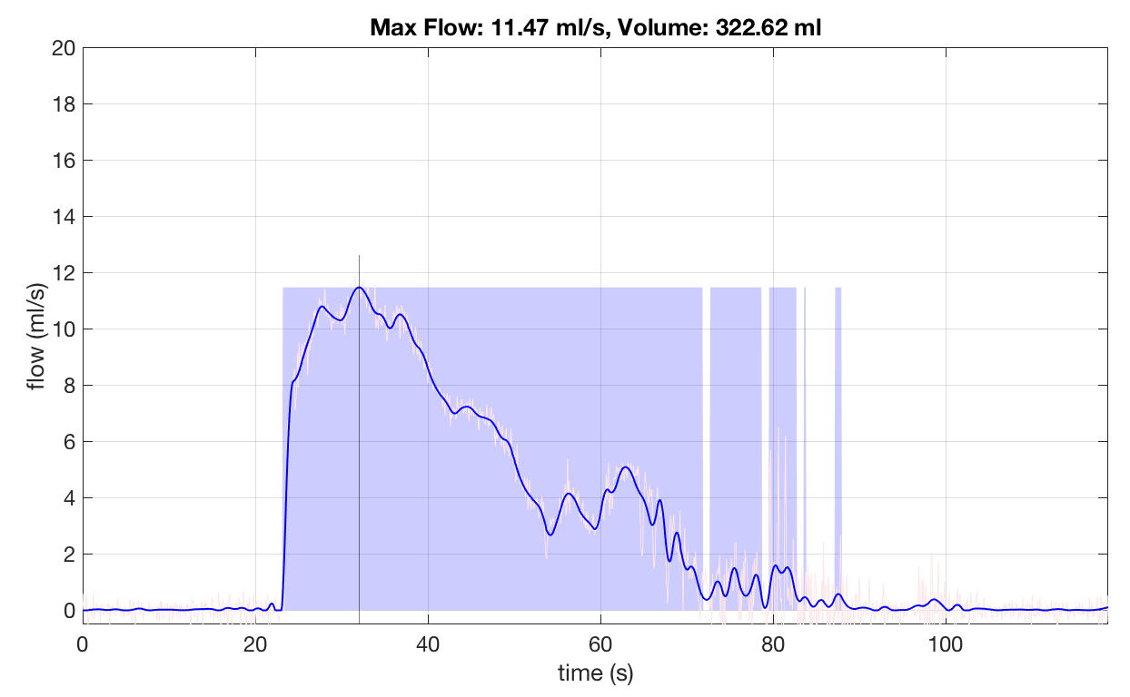 Figure 8 : Result of a typical exam done with the prototype.
The blue line is the filtered plot. The raw flow can be seen in light red. The black line tells where the max flow is and the blue regions estimates the non-zero flow (if you get several blue regions it means you stop peeing a lot in the same “go”). In the top of the plot you have the two numbers that the doctor is interested: The max flow and the total volume.
With everything working, it was time to use it! I spent 40 days using it and collected around 120 complete exams. Figure 9 shows all of them in one plot (just for the fun of it %-).
Figure 8 : Result of a typical exam done with the prototype.
The blue line is the filtered plot. The raw flow can be seen in light red. The black line tells where the max flow is and the blue regions estimates the non-zero flow (if you get several blue regions it means you stop peeing a lot in the same “go”). In the top of the plot you have the two numbers that the doctor is interested: The max flow and the total volume.
With everything working, it was time to use it! I spent 40 days using it and collected around 120 complete exams. Figure 9 shows all of them in one plot (just for the fun of it %-).
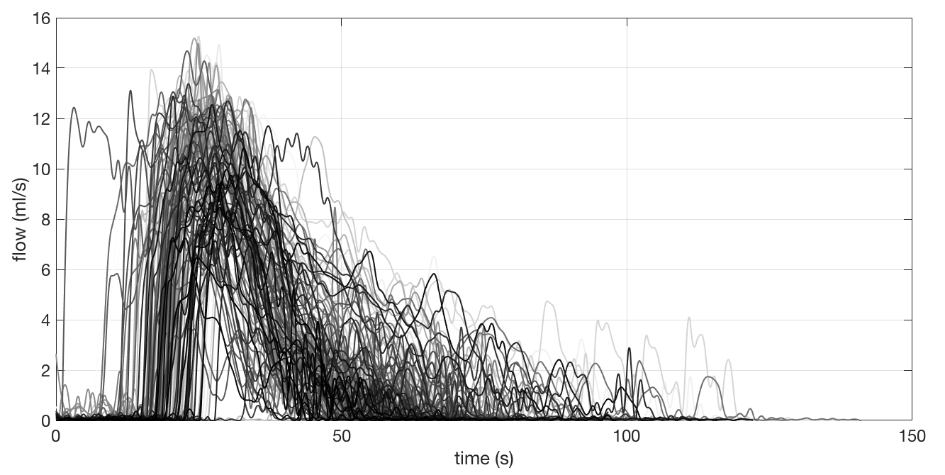 Figure 9 : 40 days of exams in one plot
Obviously, this plot is useless. To just show a lot of exams does not mean too much. Hence, what I did was to do the exams for some days without the medicine and then with the medicine. Then I separated only the max flow for each exam and plotted over time. Also, I computed the mean and the standard deviation for the points with and without the medicine and plotted in the same graph. The result is showed in figure 10.
Figure 9 : 40 days of exams in one plot
Obviously, this plot is useless. To just show a lot of exams does not mean too much. Hence, what I did was to do the exams for some days without the medicine and then with the medicine. Then I separated only the max flow for each exam and plotted over time. Also, I computed the mean and the standard deviation for the points with and without the medicine and plotted in the same graph. The result is showed in figure 10.
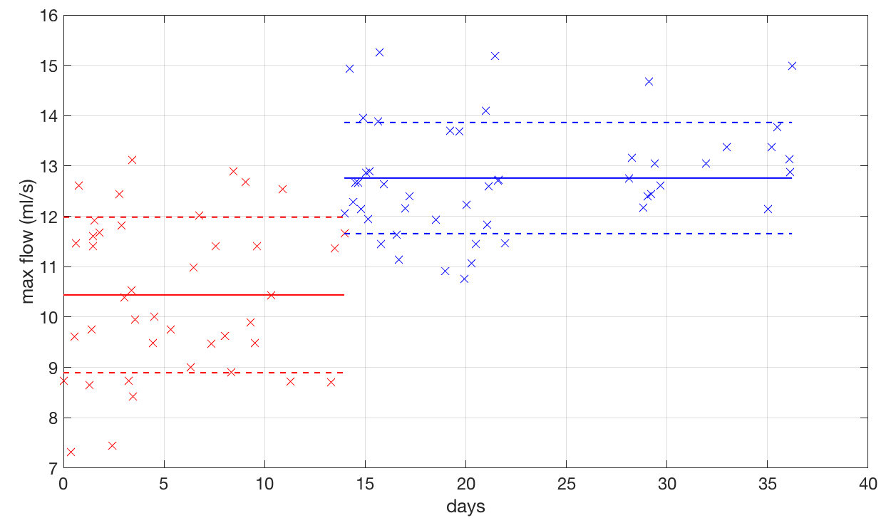 Figure 10 : Plot of max flow versus time. Red points are the results of max flow whiteout the medicine. The blue ones are the result with the medicine.
Well, as you can see, the medicine works a bit for me! The average for each situations is different and they are within more or less one standard deviation from each other. However, with this plot you can see that some times, even with the medicine, I got some low values… Those were the days I was not at my best for taking the water out of my knee. On the other hand, at some other days, even without the medicine, I was feeling like the bullet that killed Kennedy and got a good performance! In the end, statistically, I could prove that indeed the medicine was working.
Figure 10 : Plot of max flow versus time. Red points are the results of max flow whiteout the medicine. The blue ones are the result with the medicine.
Well, as you can see, the medicine works a bit for me! The average for each situations is different and they are within more or less one standard deviation from each other. However, with this plot you can see that some times, even with the medicine, I got some low values… Those were the days I was not at my best for taking the water out of my knee. On the other hand, at some other days, even without the medicine, I was feeling like the bullet that killed Kennedy and got a good performance! In the end, statistically, I could prove that indeed the medicine was working.