In this small project, I finally did what I was dreaming on doing since I started playing with the Kinect API. For those who don’t know what a Kinect is, it is a special “joystick” that Microsoft invented. Instead of holding the joystick, you move in front of it and it captures your “position”. In this project I interfaced this awesome sensor with an awesome software: blender.
Kinect
The Kinect sensor is an awesome device! It has something that is called a “depth camera”. It is basically a camera that produces an image where each pixel value is related to how far is the the actual image that the pixel represent. This is cool because, on this image, its very easy to segment a person or an object. Using the “depth” of the segmented person on the image, it is possible, although not quite easy, to identify the person’s limbs as well as their joints. The algorithm that does that is implemented on the device and consists of a very elaborated statistical manipulation of the segmented data.
Microsoft did a great job in implementing those algorithms and making them available in the Kinect API. Hence, when you install the SDK, you get commands that returns all the x,y,z coordinates of something around 25 joints of the body of the person in front of the sensor. Actually, it can return the joints of several people at the same time! Each joint relates to a link representing some limb of the person. We have, for instance, the left and right elbows, the knees, the torso, etc. The whole of the joints we call a skeleton. Hence, in short, the API returns to you, at each frame that the camera grabs, the body position of the person/people in front of the sensor! And Microsoft made It very easy to use!
With the API at hand, the possibilities are limitless! So, you just need a good environment to “draw” the skeleton of the person and you can do whatever you want with it. I can’t think of a better environment than my favorite 3D software: blender!
Blender side
Blender is THE 3D software for hobbyist like me. The main feature, in my opinion, is the python interface. Basically you can completely command blender using a python script inside the blender itself. You can create custom panel’s, custom commands and even controls (like buttons, sliders and etc). Within the panel, we can have a “timer” where you can put code that will be called in a loop without block the normal blender operations.
So, for this project, we basically have a “crash test dummy doll” made of armature bones. The special thing here is that this dummy joints and limbs are controlled by the kinect sensor! In short, we implemented a timer loop that reads the Kinect positions for each joint and set the corresponding bone coordinates in the dummy doll. The interface looks like this. There is also a “rigged” version where the bones are rigged to a simple “solid body”.
Hence, the blender file is composed basically of tree parts: the 3D body, the panel script and a Kinect interface script. The challenge was to interface the Kinect with python. For that I used two awesome libraries: pygame and pykinect2. I’ll talk about them in the next section. Unfortunately, the libraries did not like the python environment of blender and they were unable to run inside the blender itself. The solution was to implement a client server structure. The idea was to implement a small Inter Process Communication (IPC) system with local sockets. The blender script would be the client (sockets are ok in blender 😇) and a terminal application would run the server.
Python side
For the python side of things we have basically the client and the server I just mentioned. They communicate via socket to implement a simple IPC system. The client is implemented in the blender file and consists of a simple socket client that opens a connection to a server and reads values. The protocol is extremely simple. The values are sent in order. First, all the x’s coordinates of the joints, then y’s and then z’s. So, the client is basically a loop that reads joint coordinates and “plots” them accordingly in the 3D dummy doll.
The server is also astonishingly simple. It has two classes: the KinectBodyServer class and the BodyGameRuntime class. In the first one we have a server of body position that implements the socket server and literally “serves body positions” to the client. It does so by instantiating a Kinect2 object and, using the PyKinect2 API, asks for joint positions to the device. The second class is the pygame object that takes care of showing the screen with the camera image (the RGB camera) and handling window events like Ctrl+C, close, etc. It also instantiates the body server class to keep pooling for joint positions and to send them to the client.
Everything works synchronously. When the client connects to the server, it expects to keep receiving joint positions until the server closes and disconnects. The effect is amazing (see video bellow). Now, you can move in front the sensor and see the blender dummy doll imitate your moves 😀!
Motion Capture
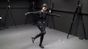
Not long ago, big companies spent a lot of money and resources to “motion capture” a person’s body position. It involved dressing the actor with a suit full of small color markers and filming it from several angles. A technician would then manually correct the captured position of each marker.
(source: https://www.sp.edu.sg/mad/about-sd/facilities/motion-capture-studio)
Now, if you don’t need extreme precision on the positions, an inexpensive piece of hardware like Kinect and a completely free software like blender (and the python libraries) can do the job!
Having fun
The whose system in action can be viewed in the video bellow. The capture was made in real time. The image of the camera and the position of the skeleton have a little delay that is negligible. That means that one can use, even with the IPC communication delay and all, as a game joystick.
Conclusions
As always, I hope you liked this post. Feel free to share and comment. The files are available at GitHub as always (see reference). Thank you for reading!!!
Wavefront sensing is the act of sensing a wave front. As useless as this sentence gets, it is true and we perform this action with a wavefronts sensor… But if you bare with me, I promise that its going to be one of the coolest mix of science and technology that you will hear about! Actually, I promise that it would be even poetic, since that, in this post, you will learn why the stars twinkle in the sky!
Just a little disclaim before I start: Im not an optical engineer and I understand very little about the subject. This post is just myself sharing my enthusiasm about this amazing subject.
Well, first of all, the word sensing just mean “measure”. Hence, wavefront sensing is the act of measure a wave front with a wavefront sensor. To understand what a wavefront measurement is, let me explain what a wavefront is and why one would want to measure it. It has to do with light. In a way, wavefront measurement is the closest we can get from measuring the “shape” of a light wave. The first time I came across this concept (here in the Geneva observatory) I asked myself: “What does that mean? Doesn’t light has the form of its source??”. I guess thats a fair question. In the technical use of the term measurement, we consider here that we want to measure the “shape” of the wave front that was originated in a point source of light very far away. You may say: “But thats just a plain wave!” and you would be right if we were in a complete homogeneous environment. If that were the case, we would have nothing to measure %-). So, what happens when we are in a non-homogenous medium? The answer is: The wavefront gets distorted, and we got to measure how distorted it is! When light propagates as a plain wave and it passes through an non-homogeneous medium, part of its wavefront slows down and others don’t. That creates a “shape” in the phase of the wavefront. Because of the difference in the index of refraction of the medium, in some locations, the oscillation of the electromagnetic arrives a bit earlier and some other it arrives a bit later. This creates a diferente in phase at each point in space. The following animation tries to convey this idea.
Figure 1: Wavefront distorted by a medium
As we see in the animation, the wavefront is plain before reaching the non-homogeneous medium (middle part). As it passes through the medium, it exits with a distorted wavefront. Since the wavefront is always traveling in a certain direction, we are only interested in measure it in a plane (in the case of the animation, a line) perpendicular to its direction of propagation.
In the animation above, a measurement at the left side would result in a constant value since, for all “y” values of the figure, the wave arrives at the same time. If we measure at the left side we get something like this
Figure 2: Wavefront measurement for the medium showed in Figure 1
Of course that, in a real wavefront, the measurement would be 2D (so the plot would be a surface plot).
An obvious question at this point is: Why someone would want to measure a wavefront? There is a lot os applications in optics that requires the measurement of a wavefront. For instance, lens manufacturer would like to know if the shape of the lenses they manufactured is within a certain specification. So they shoot a plane wavefront through the lens of the glass and measure the deformation in the wavefront causes by the lens. By doing that, they measure the lens properties like astigmatism, coma and etc. Actually, did you ever asked yourself where those names (defocus, astigmatism, coma) came from? Nevertheless, one of the the most direct use of this wavefront measuring is in astronomy! Astronomers like to look at the stars. But the stars are very far away and, for us, they are an almost perfect point source of light. That means that we should receive a plain wave here right? Well if we did we have nothing to breath! Yes, the atmosphere is the worst enemy of the astronomers (thats why they spend millions and millions to put a telescope in orbit). When the light of the star or any object passes through the atmosphere, it gets distorted. Its wavefront make the objet’s image swirl and stretch randomly. Worst then that, the atmosphere is always changing its density due to things like wind, clouds and difference in temperatures. So, the wavefront follows this zigzags and THAT is why the stars twinkle in the sky! (I promise didn’t I? 😃) So, the astronomers build sophisticated mechanisms using adaptive optics to compensate for this twinkling and that involves, first of all, to measure the distortion of the wavefront.
Wavefront measurement
So, how the heck do we measure this wavefront? We could try to put small light sensors in an array and “sense” the electromagnetic waves that arrives at them… But light is pretty fast. It would be very very difficult to measure the time difference between the rival of the light in one sensor compared to the other (the animation in figure 1 is like a SUPER MEGA slow motion version of the reality). So, we have to be clever and appeal to the “jump of the cat” (expression we use in Brazil to mean a very smart move to solve a problem).
In fact, the solution is very clever! Although there are different kinds of wavefront sensors, the one I will explain here is called Shack–Hartmann wavefront sensor. The ideia is amazingly simple. Instead of measuring directly the phase of the wave (that would be difficult because light travels too fast) we could measure the “inclination” or the local direction of propagation of the wavefront. Now, instead of an array of light sensors that would try to measure the arrival time, we make an array of sensors that measure the local direction of the wavefront. With this information it is possible to recover the phase of the wavefront, but that is a technical detail. So, in summary, we only need to measure the angles of arrival of the wavefront. Figure 3 tries to exemplify that I mean:
Figure 3: Exemple of measurement of direction of arrival, instead of time of arrival.
Each horizontal division in the figure is a “sub-aperture” where we measure the inclination of the wavefront. Basically we measure the angle of arrival, instead of the time of arrival (or phase of arrival). If we do those sub-apertures small enough, we can reconstruct a good picture of the wavefront. Remember that for real wavefronts we have a plane, so we should measure TWO angles of arrival for each sub-aperture (the angle in x and the angle in y, considering that z is the direction of propagation).
At this point you might be thinking: “Wait… you just exchanged 6 for 12/2! How the heck do we measure this angle of arrival? It seems that this is far more difficult then to measure the phase itself!”. Now its time to get clever! The idea is to put a small camera in each sub aperture. Each tiny camera will be equipped with a tiny little lens to focus the portion of the wavefront to a certain pixel of this tiny camera! Doing that, at each camera, depending on the angle of arrival, the lens will focus the locally plain wave to a certain region of the camera dependent on the direction its traveling. That will make each camera see a small region with bright pixels. If we measure where those pixels are in relation to the center of the tiny camera, we have the angle of arrival!!! You might be thinking that its crazy to manufacture small cameras and small lenses in a reasonable packing. Actually, what happens is that we just have the tiny lenses in front of a big CCD. And it turns out that we don’t need hight resolution cameras in each sub-aperture. A typical wavefront sensor has 32×32 sub apertures, each one with a 16×16 grid os pixels. That is enough to give a very good estimation of the wavefront. Figure 4 shows a real image of a wavefront sensor.
Figure 4: Sample image from a real wavefront sensor
Simulations!
The principle is so simple that we can simulate it in several different ways. The first one is using the “light ray approach” for optics. This principle is the one we learn in college. Its the famous one that they put a stick figure on one side of a lens or a mirror and them draw some lines representing the light path. The wavefront sensor would be a bit more complex to draw, so we use the computer. Basically what I did was to make a simple blender file that contains a light source, something for the light to pass through (atmosphere) and the sensor itself. The sensor is just an 2D array of small lenses (each one made up by two spheres intersected) and a set of planes behind each lens to receive the light. We then set up a camera between the lenses and the planes to be able to render the array of planes, as they would be the CCD detectors of the wavefront sensor. Now we have to set the material for each object. The “detectors” must be something opaque so we could see the light focusing on it. The atmosphere have to be some kind of glass (with a relatively low index of refraction). The lenses also have glass as its material, but their index of refraction must be carefully adjusted so the focus of each one can be exactly on the detectors plane. Thats pretty much it (see figure 5).
Figure 5: Setup for simulating a wavefront sensor in blender
To simulate the action, we move the “atmosphere” object back and forth and render each step. As light passes through the object, it diffracts it. That changes the direction of the light rays and simulates the wavefront being deformed. The result is showed in figure 6.
Figure 6: Render of the image on the wavefront sensor as we move the atmosphere simulating the real time reformation of the wavefront.
Another way of simulating the wavefront sensor is to simulate the light wave itself passing through different mediums, including the leses themselves and driving at some absorbing material (to emulate the detectors). That sounds kind of hardcore simulation stuff, and it kind of is. But, as I said in the “about” of this blog, I’m curious and hyperactive, so here we go: Maxwells equations simulation of a 1D wavefront sensor. To do that simulation, I used a code that I did a couple of yeas back. I’ll make a post about it some day. It is an implementation of a FD-TD (Finite Diferences in the Time Domain) method. This is a numerical method to solve partial differential equations. Basically, you set up your environment as a 2D grid with sources of electromagnetic field, material of each element on the grid and etc. Then, you run the interactive method to see the electromagnetic fields propagating. Anyway, I put some layers of conductive material to contain the wave is some points and to emulate the detector. Then I added a layer with small lenses with the right refraction index to emulate the sub-apartures. Finally, I put a monochromatic sinusoidal source in one place and pressed run. Voilá! You can see the result in the video bellow.
The video contains the explanation of each element and, as you can see, the idea of a wavefront sensor is so brilliantly simple that we can simulate it at the Maxwells equation level!
DIY (physical) experiment
To finish this post, let me show you that you can even build your own wavefront sensor “mockup” at home! What I did in this experiment was to build a physical version of the Shack–Hartmann principle. The idea is to use a “blank wall” as detector and a webcam to record the light that arrives at the wall. This way I can simulate a giant set of detectors. Now the difficult part: the sub-aperure lenses… For this one, I had to make the cat jump. Instead of an array of hundreds of lenses in front of the “detector wall”, I uses a toy laser that comes with those diffraction crystals that projects “little star-like patterns” (see figure 7).
Figure 7: 1 – Toy laser (black stick) held in place. 2 – green “blank wall”. 3 – Diffraction pattern that generates a regular set of little dots.
With this setup, it was time to do some coding. Basically I did some Matlab functions to capture the webcam image of the wall with the dots. On those functions I setup some calibration computations to compensate for the shape and place of the dots on the wall (see video bellow). That calibration will tell me where the “neutral” atmosphere will project the points (centers of the sub apertures). Them, for each frame, I capture and process the image from the webcam. For each image, I compute the position of the processed centers with respect to the calibrated ones. With this procedure, I have, for each dot, a vector that points form the center to where it is. That is exactly the wavefront direction that the toy laser is emulating!
After that, it was a matter of having fun with the setup. I put all kinds of transparent materials in front of the laser and saw the “vector field” of the wavefront directions on screen. I even put my glasses and were able to see the same pattern the optical engineering saw when they were manufacturing the lenses! With a bit of effort I think I could even MEASURE (poorly of course) the level of astigmatism of my glasses!
The code is available in GitHub[2] but basically the loop consists in process each frame and show the vector field of the wavefront.
DIY projects are awesome for understanding theoretical concepts. In this case, the mix of simulation and practical implementation made very easy to understand how the device works. The use of the diffraction crystal in toy lasers is thought to be original, but I didn’t research a lot. If you know any experiment that uses this same principle, please let me know in the comments!
Again, thank you for reading until here! Feel free to comment o share this post. If you are an optical engineer, please correct me at any mistake I might have made on this post. It does not intend to teach about optics, but rather to share my passion for this subject that I know so little!
Thank you for reading this post. I hope you liked it and, as always, feel free to comment, give me feedback, or share if you want! See you in the next post!
This post is about health. Actually, its about a little project that implements a medical device called Uroflowmeter (not sure if that is the usual English word). Its a mouth full name to mean “little device that measures the flow of pee” (yes, pee as in urine 😇).
Last year I had to perform an exam called Uroflowmetry (nothing serious, a lot people do that exam). The doctor said that, as the name implies, I had to measure “how fast I pee”. Technically it measures the flow of urine that flows when you urinate. At the time I thought to myself: “How the heck will he do that?”. Maybe be it was using a very sophisticated device, I didn’t know. Then he explained to me that I had to pee in a special toilet hooked up to a computer. He showed me the special device and left the room (it would be difficult if he stayed and watched hehehehehe). I didn’t see any sign of ultra technology anywhere. Then, I got the result and was nothing serious.
The exam result is a plot of flow vs time. Figure 1 shows an example of such exam. Since my case was a simple one, the only thing that matted in that exam was the maximum value. So, for me, the result was a single number (but I still had to do the whole exam and get the whole plot).
Figure 1 : Sample of a Uroflowmetry result[3]
Then, he prescribe a very common medicine to improve the results and told me that I would repeat the exam a couple of days later. After about 4 or 5 days I returned to the second exam. I repeated the whole process and peed on the USD $10,000.00 toilet. This time I did’t feel I did my “average” performance. I guess some times you are nervous, stressed or just not concentrated enough. So, as expected, the results were not ultra mega perfect. Long story short, the doctor acknowledge the result of the exam and conducted the rest of the visit (I’m fine, if you are wondering heheheh).
That exam got me thinking that it (the exam) did not capture the real “performance” of the act, by measuring only one flow. I might had notice some improvement with the medication, but I wasn’t so sure. So, how to be sure? Well, if only I could repeat the exam several times in several different situations… By doing that I could see the performance in average. I thought so seriously about that, that I asked the clinic how much does the exam costs. The lady in the desk said that it around $100,00 Brazil Reais ($30.00 USD, more or less in today’s rate). That was a bummer… The health insurance won’t simply pay lots of exams for me and if I were to make, say, 10 exams, it would cost me one thousand Brazil Reais. Besides, I would still have only 10 data points.
The project
Thinking about that, maybe I could measure it myself…? Then I decided to make my own “Urine flow meter”. it would be a Hardware / Software project, so I mediately though of using an Arduino (figure 2). The trick part is to measure the flow of something like urine. The solution I came up was to make an Arduino digital scale to measure the weight of the pee while I’m peeing on it (awkward or disgusting as it sounds %-). Then, I could measure the weight in real time at each, say, 20 to 50ms. Knowing the density of the fluid I’m testing I could compute the flow by differentiating the time measurement. Google told me that the density of urine is about 1.0025mg/l (if you are curious, its practically water actually). Later on I discovered that, that is exactly how some machine works, including the one I did the exams.
Figure 2 : Arduino board
First I had to make the digital scale, so I used a load cell that had the right range for this project. The weight of the urine would range from 0 to 300~500mg more or less, so I acquire a 2Kg range load cell (Figure 3 and 4). I disassemble an old kitchen scale to use the “plate” that had the right space to hold the load cell and 3D printed a support in a heavy base to avoid errors in the measurements due to the flexing of the base. For that, I used a heavy ceramic tile that worked very well. The cell “driver” was an Arduino library called HX711. There is a cool youtube tutorial showing how to use this library [1].
Figure 3 : Detail of the load cell used to make the digital scale.
Figure 4 : Loadcell connected to the driver HX711
The next problem was how to connect to the computer!!! This is not a regular project that you can assemble everything on your office and do tests. Remember that I had do pee on the hardware! I also didn’t want to bring a notebook to the bathroom every time I want to use it! the solution was to use a wifi module and communicate wirelessly. Figure 5 shows the module I used. Its an ESP8266. Now I could bring my prototype to the bathroom and pee on it while the data would be sent to the computer safely.
Figure 5 : ESP8266 connection to the Arduino board.
Figure 6 : More pictures of the prototype
Once built, I had to calibrate it very precisely. I did some tests to measure the sensibility of the scale. I used an old lock and a small ball bearing to calibrate the scale. I went to the laboratory of Metrology at my university and a very nice technician in the lab (I’m so sorry I forgot his name, but he as very very kind) measures the weights of the lock and the ball bearing in a precision scale. Then I started to do some tests (see video bellow)
The last thing to make the prototype 100% finished was to have a funnel that had the right size. So I 3D printed a custom size funnel I could use (figure 7).
Figure 7: Final prototype ready to use
Once calibrated and ready to measure weights in real time, It was time to code the flow calculation. At first, this is a straight forward task, you just differentiate the measurements in time. Something like
$$
\begin{equation}
f[n] = \frac{{w[n – 1] – w[n]}}{{\rho \Delta t}}
\end{equation}
$$
Where \(f[n]\) and \(w[n]\) are the flow and weight at time \(n\). \(\rho\) is the density and \(\Delta t\) is the time between measurements.
Unfortunately, that simple procedure is not enough to generate the plot I was hoping for. That’s because the data has too much noise. But I teach DSP, so I guess I could do some processing right 😇? Well I took the opportunity to test several algorithms (they are all in the source code at GitHub[2]). I won’t dive into details here about each one. The important thing is that the noise was largely because of the differentiation process so I tested filtering before and after compute the differentiation. The method that seemed to give better results was the spline method. Basically I got the flow data and averaged \(N\) fitted downsampled data with a spline. One sample of the results can be seen in figure 8.
Figure 8 : Result of a typical exam done with the prototype.
The blue line is the filtered plot. The raw flow can be seen in light red. The black line tells where the max flow is and the blue regions estimates the non-zero flow (if you get several blue regions it means you stop peeing a lot in the same “go”). In the top of the plot you have the two numbers that the doctor is interested: The max flow and the total volume.
With everything working, it was time to use it! I spent 40 days using it and collected around 120 complete exams. Figure 9 shows all of them in one plot (just for the fun of it %-).
Figure 9 : 40 days of exams in one plot
Obviously, this plot is useless. To just show a lot of exams does not mean too much. Hence, what I did was to do the exams for some days without the medicine and then with the medicine. Then I separated only the max flow for each exam and plotted over time. Also, I computed the mean and the standard deviation for the points with and without the medicine and plotted in the same graph. The result is showed in figure 10.
Figure 10 : Plot of max flow versus time. Red points are the results of max flow whiteout the medicine. The blue ones are the result with the medicine.
Well, as you can see, the medicine works a bit for me! The average for each situations is different and they are within more or less one standard deviation from each other. However, with this plot you can see that some times, even with the medicine, I got some low values… Those were the days I was not at my best for taking the water out of my knee. On the other hand, at some other days, even without the medicine, I was feeling like the bullet that killed Kennedy and got a good performance! In the end, statistically, I could prove that indeed the medicine was working.
Conclusions
I was very happy that I could do this little project. Of course that this results can’t be used as a definite medical asset. I’m not a physician, so I’m not qualified to take any action whatsoever based on those results. I’ll show it to my doctor and he will decide what to do with them. The message I would like to transmit with it to my audience (students, friend, etc) is that, what you learn at the university is not just “stuff to pass on the exams”. They are things that you learn that can help a lot if you really understand them. This project didn’t need any special magical skill! Arduino is simple to use, the sensor and the wifi ESP have libraries. The formula to compute flow from weight is straight forward. Even the simple signal filtering that I used (moving average) got good results for the max flow value. Hence, I encourage you, technology enthusiast to try things out! Use the knowledge that you acquired in your undergrad studies! Its not only useful, its fun! Who would have thought that, at some point in my life, I would pee on one of my projects!!! 😅
Thank you for reading this post. I hope you liked it and, as always, feel free to comment, give me feedback, or share if you like! See you in the next post!
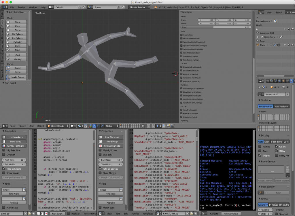 Hence, the blender file is composed basically of tree parts: the 3D body, the panel script and a Kinect interface script. The challenge was to interface the Kinect with python. For that I used two awesome libraries: pygame and pykinect2. I’ll talk about them in the next section. Unfortunately, the libraries did not like the python environment of blender and they were unable to run inside the blender itself. The solution was to implement a client server structure. The idea was to implement a small Inter Process Communication (IPC) system with local sockets. The blender script would be the client (sockets are ok in blender 😇) and a terminal application would run the server.
 (source: https://www.sp.edu.sg/mad/about-sd/facilities/motion-capture-studio)

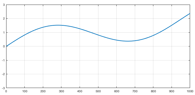
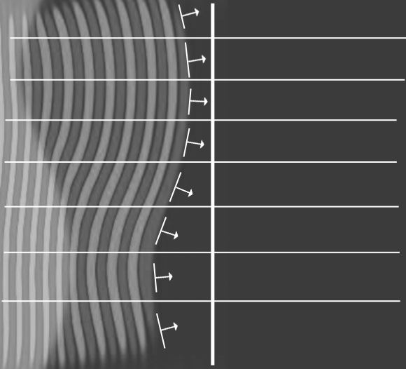
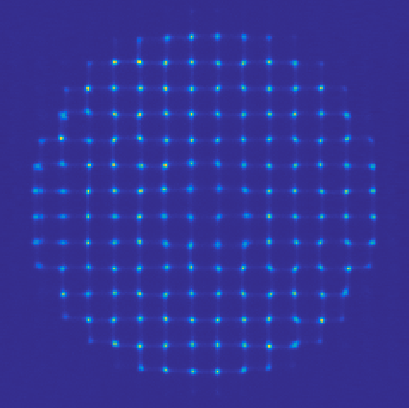
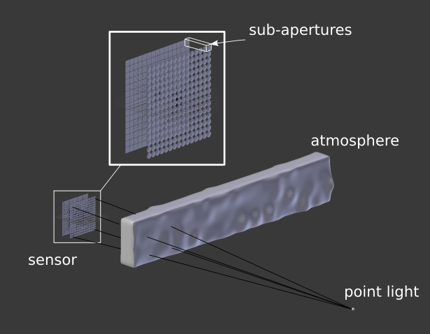
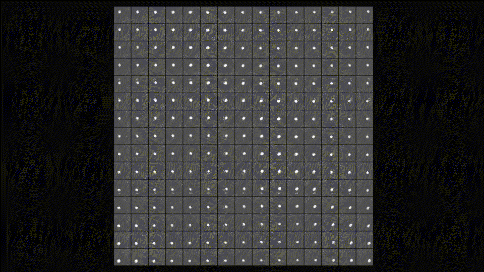
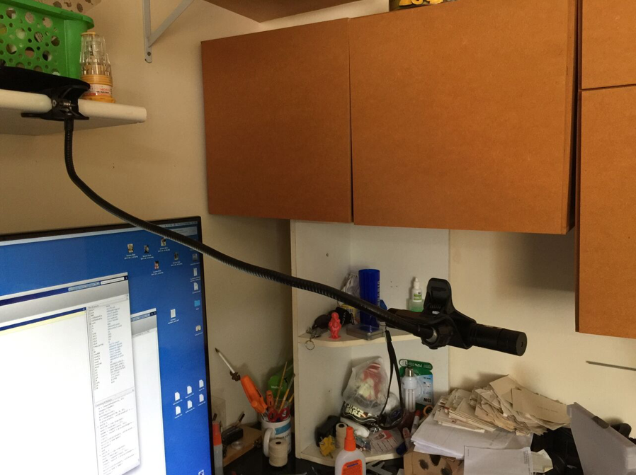
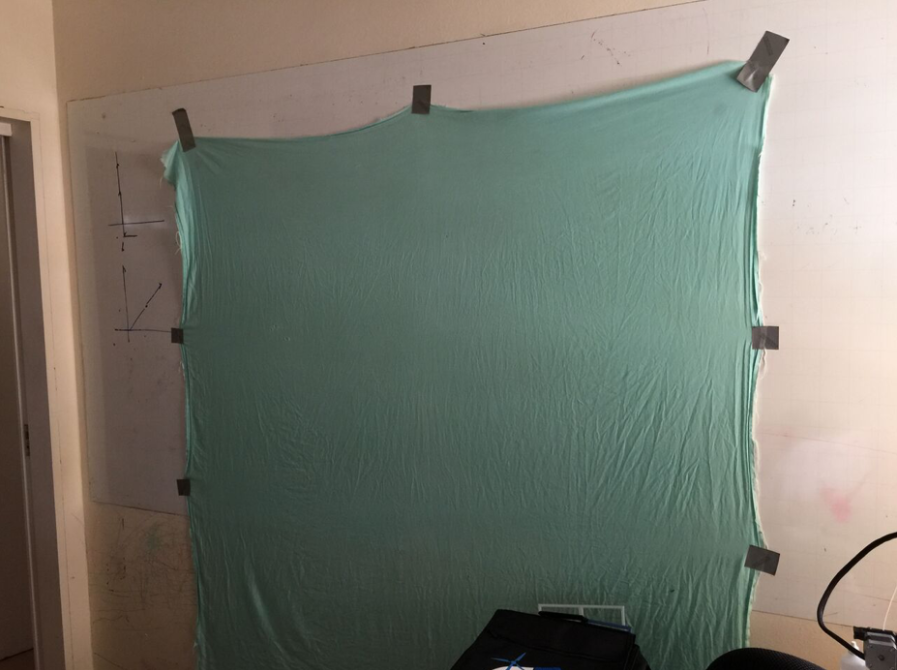
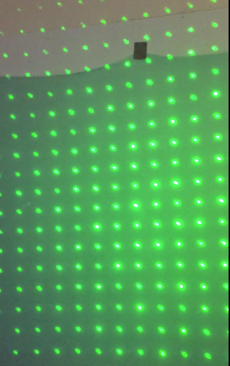
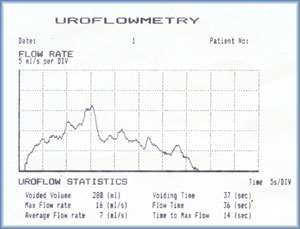 Figure 1 : Sample of a Uroflowmetry result[3]
Then, he prescribe a very common medicine to improve the results and told me that I would repeat the exam a couple of days later. After about 4 or 5 days I returned to the second exam. I repeated the whole process and peed on the USD $10,000.00 toilet. This time I did’t feel I did my “average” performance. I guess some times you are nervous, stressed or just not concentrated enough. So, as expected, the results were not ultra mega perfect. Long story short, the doctor acknowledge the result of the exam and conducted the rest of the visit (I’m fine, if you are wondering heheheh).
Figure 1 : Sample of a Uroflowmetry result[3]
Then, he prescribe a very common medicine to improve the results and told me that I would repeat the exam a couple of days later. After about 4 or 5 days I returned to the second exam. I repeated the whole process and peed on the USD $10,000.00 toilet. This time I did’t feel I did my “average” performance. I guess some times you are nervous, stressed or just not concentrated enough. So, as expected, the results were not ultra mega perfect. Long story short, the doctor acknowledge the result of the exam and conducted the rest of the visit (I’m fine, if you are wondering heheheh).
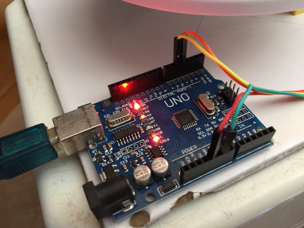 Figure 2 : Arduino board
First I had to make the digital scale, so I used a load cell that had the right range for this project. The weight of the urine would range from 0 to 300~500mg more or less, so I acquire a 2Kg range load cell (Figure 3 and 4). I disassemble an old kitchen scale to use the “plate” that had the right space to hold the load cell and 3D printed a support in a heavy base to avoid errors in the measurements due to the flexing of the base. For that, I used a heavy ceramic tile that worked very well. The cell “driver” was an Arduino library called HX711. There is a cool youtube tutorial showing how to use this library [1].
Figure 2 : Arduino board
First I had to make the digital scale, so I used a load cell that had the right range for this project. The weight of the urine would range from 0 to 300~500mg more or less, so I acquire a 2Kg range load cell (Figure 3 and 4). I disassemble an old kitchen scale to use the “plate” that had the right space to hold the load cell and 3D printed a support in a heavy base to avoid errors in the measurements due to the flexing of the base. For that, I used a heavy ceramic tile that worked very well. The cell “driver” was an Arduino library called HX711. There is a cool youtube tutorial showing how to use this library [1].
 Figure 3 : Detail of the load cell used to make the digital scale.
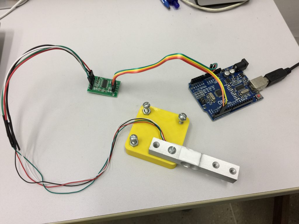 Figure 4 : Loadcell connected to the driver HX711
The next problem was how to connect to the computer!!! This is not a regular project that you can assemble everything on your office and do tests. Remember that I had do pee on the hardware! I also didn’t want to bring a notebook to the bathroom every time I want to use it! the solution was to use a wifi module and communicate wirelessly. Figure 5 shows the module I used. Its an ESP8266. Now I could bring my prototype to the bathroom and pee on it while the data would be sent to the computer safely.
Figure 4 : Loadcell connected to the driver HX711
The next problem was how to connect to the computer!!! This is not a regular project that you can assemble everything on your office and do tests. Remember that I had do pee on the hardware! I also didn’t want to bring a notebook to the bathroom every time I want to use it! the solution was to use a wifi module and communicate wirelessly. Figure 5 shows the module I used. Its an ESP8266. Now I could bring my prototype to the bathroom and pee on it while the data would be sent to the computer safely.
 Figure 5 : ESP8266 connection to the Arduino board.
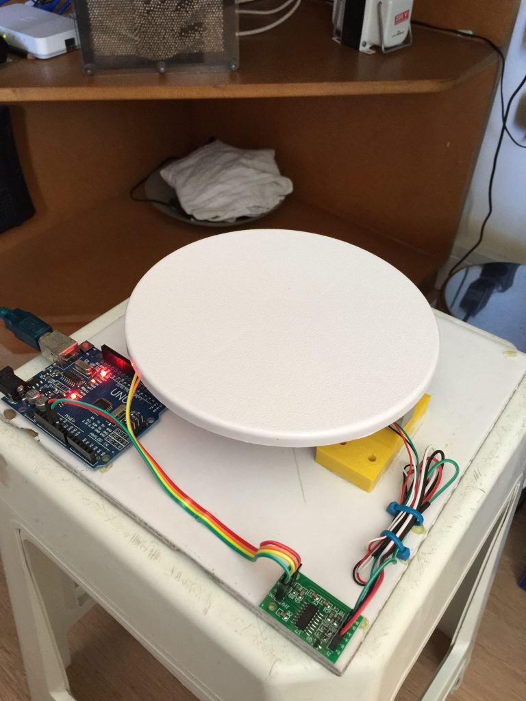
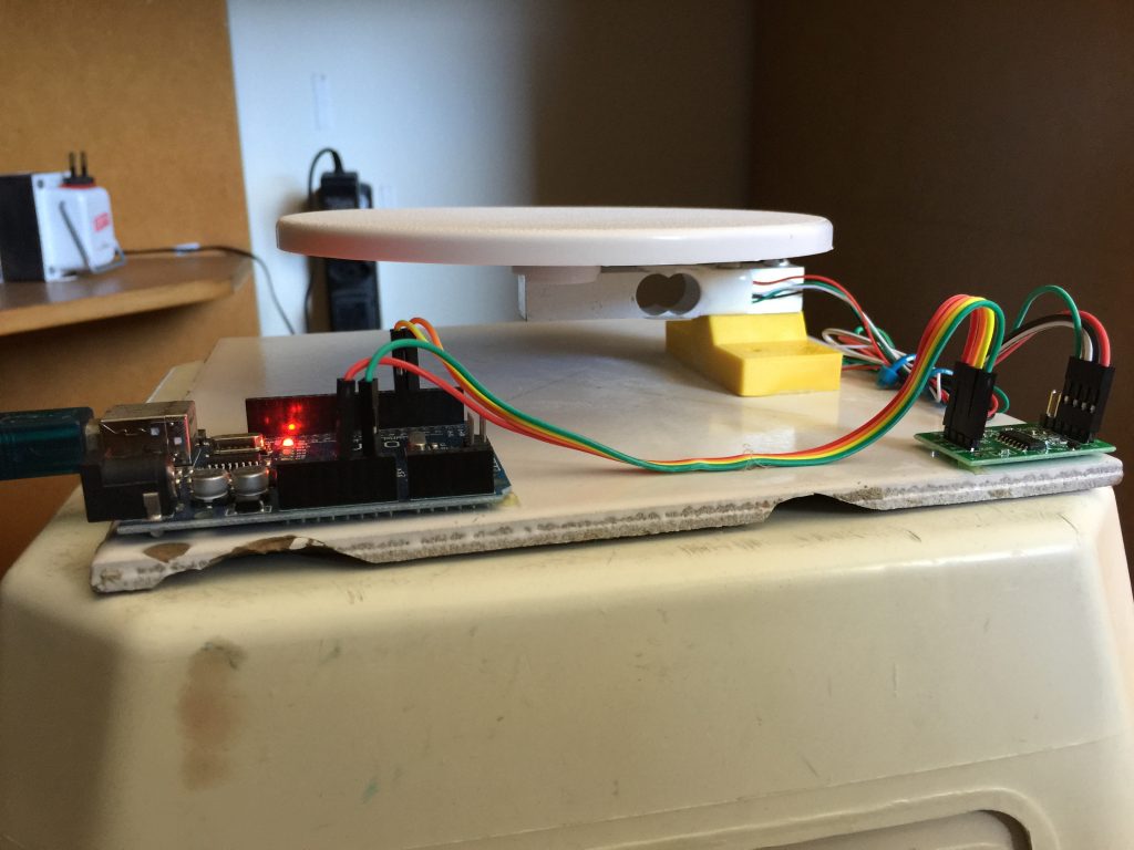
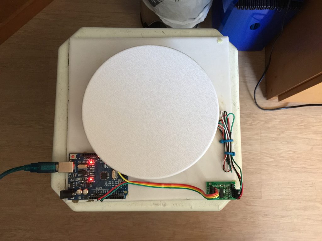 Figure 6 : More pictures of the prototype
Once built, I had to calibrate it very precisely. I did some tests to measure the sensibility of the scale. I used an old lock and a small ball bearing to calibrate the scale. I went to the laboratory of Metrology at my university and a very nice technician in the lab (I’m so sorry I forgot his name, but he as very very kind) measures the weights of the lock and the ball bearing in a precision scale. Then I started to do some tests (see video bellow)
The last thing to make the prototype 100% finished was to have a funnel that had the right size. So I 3D printed a custom size funnel I could use (figure 7).
Figure 6 : More pictures of the prototype
Once built, I had to calibrate it very precisely. I did some tests to measure the sensibility of the scale. I used an old lock and a small ball bearing to calibrate the scale. I went to the laboratory of Metrology at my university and a very nice technician in the lab (I’m so sorry I forgot his name, but he as very very kind) measures the weights of the lock and the ball bearing in a precision scale. Then I started to do some tests (see video bellow)
The last thing to make the prototype 100% finished was to have a funnel that had the right size. So I 3D printed a custom size funnel I could use (figure 7).
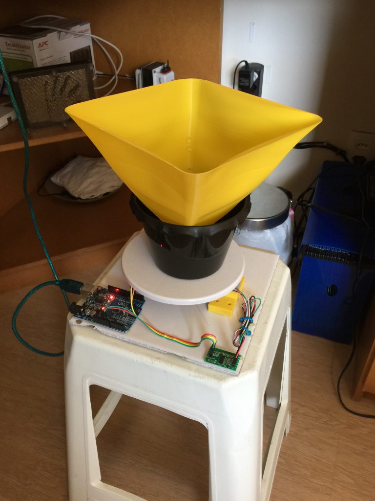
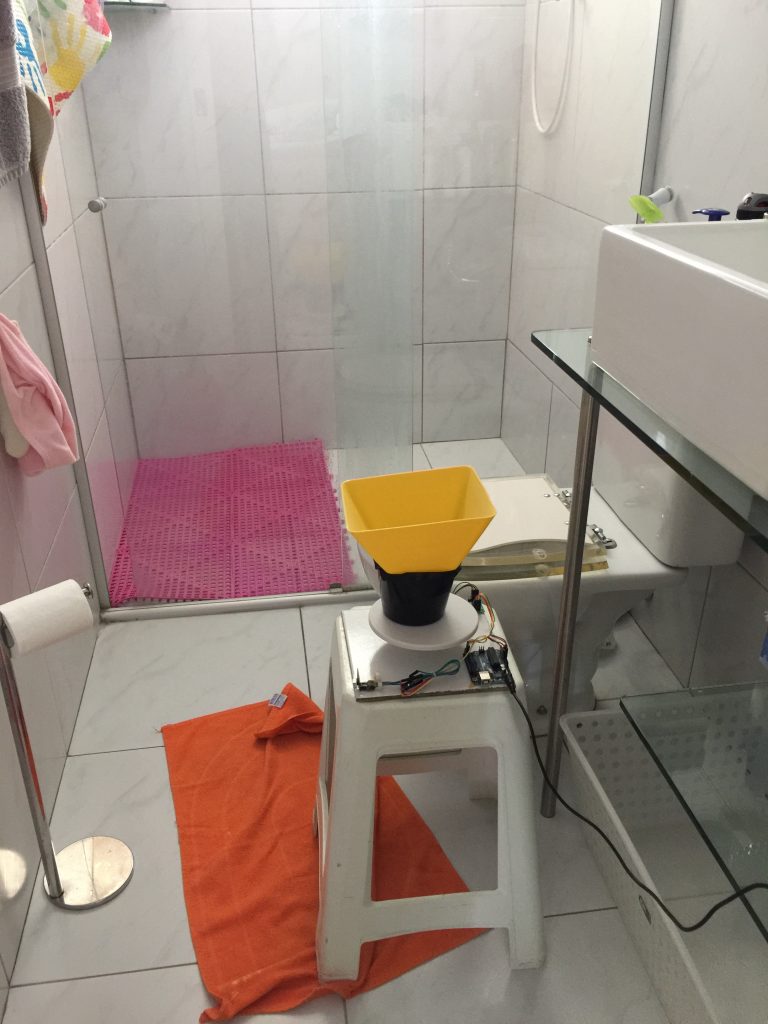 Figure 7: Final prototype ready to use
Once calibrated and ready to measure weights in real time, It was time to code the flow calculation. At first, this is a straight forward task, you just differentiate the measurements in time. Something like
$$
\begin{equation}
f[n] = \frac{{w[n – 1] – w[n]}}{{\rho \Delta t}}
\end{equation}
$$
Where \(f[n]\) and \(w[n]\) are the flow and weight at time \(n\). \(\rho\) is the density and \(\Delta t\) is the time between measurements.
Figure 7: Final prototype ready to use
Once calibrated and ready to measure weights in real time, It was time to code the flow calculation. At first, this is a straight forward task, you just differentiate the measurements in time. Something like
$$
\begin{equation}
f[n] = \frac{{w[n – 1] – w[n]}}{{\rho \Delta t}}
\end{equation}
$$
Where \(f[n]\) and \(w[n]\) are the flow and weight at time \(n\). \(\rho\) is the density and \(\Delta t\) is the time between measurements.
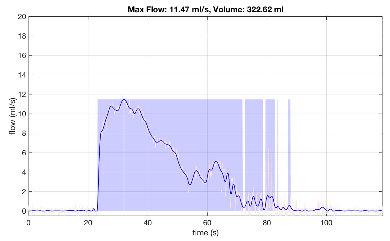 Figure 8 : Result of a typical exam done with the prototype.
The blue line is the filtered plot. The raw flow can be seen in light red. The black line tells where the max flow is and the blue regions estimates the non-zero flow (if you get several blue regions it means you stop peeing a lot in the same “go”). In the top of the plot you have the two numbers that the doctor is interested: The max flow and the total volume.
With everything working, it was time to use it! I spent 40 days using it and collected around 120 complete exams. Figure 9 shows all of them in one plot (just for the fun of it %-).
Figure 8 : Result of a typical exam done with the prototype.
The blue line is the filtered plot. The raw flow can be seen in light red. The black line tells where the max flow is and the blue regions estimates the non-zero flow (if you get several blue regions it means you stop peeing a lot in the same “go”). In the top of the plot you have the two numbers that the doctor is interested: The max flow and the total volume.
With everything working, it was time to use it! I spent 40 days using it and collected around 120 complete exams. Figure 9 shows all of them in one plot (just for the fun of it %-).
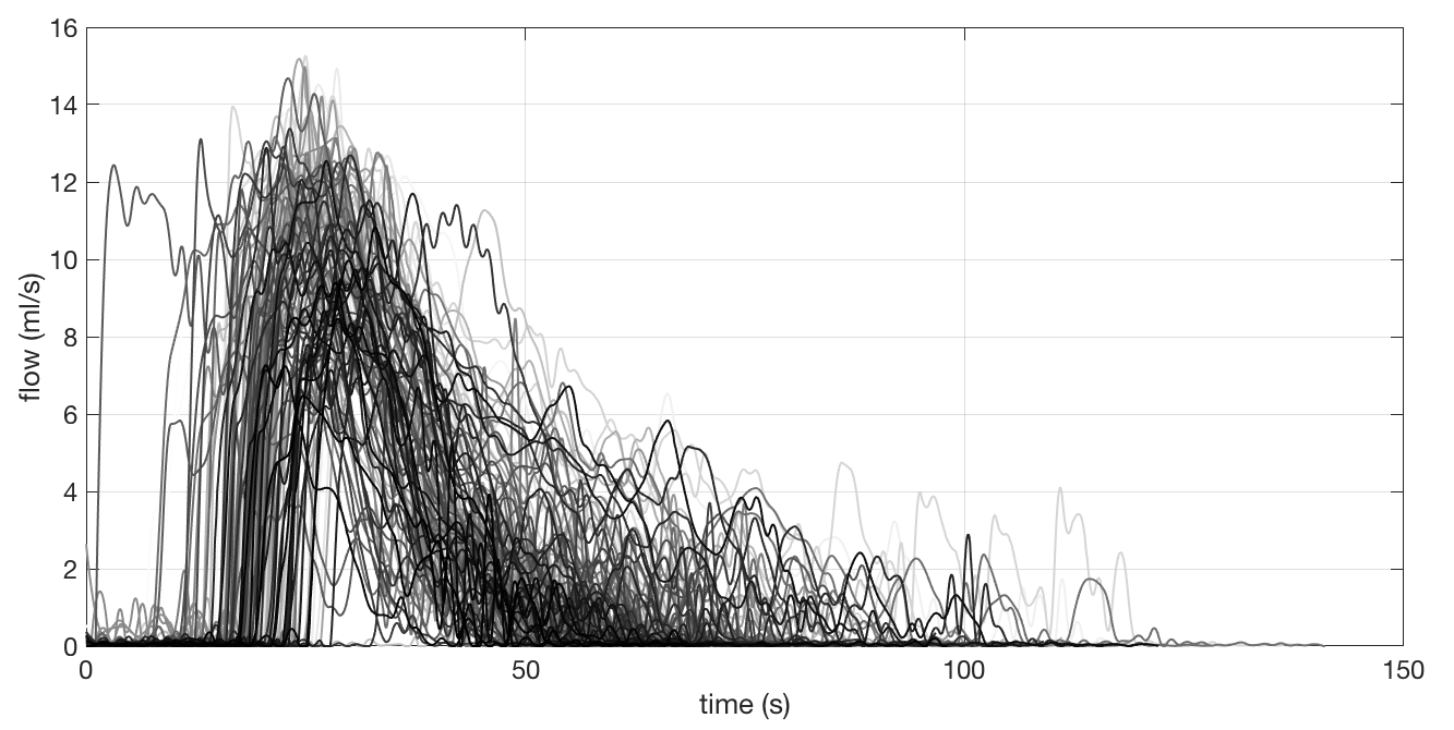 Figure 9 : 40 days of exams in one plot
Obviously, this plot is useless. To just show a lot of exams does not mean too much. Hence, what I did was to do the exams for some days without the medicine and then with the medicine. Then I separated only the max flow for each exam and plotted over time. Also, I computed the mean and the standard deviation for the points with and without the medicine and plotted in the same graph. The result is showed in figure 10.
Figure 9 : 40 days of exams in one plot
Obviously, this plot is useless. To just show a lot of exams does not mean too much. Hence, what I did was to do the exams for some days without the medicine and then with the medicine. Then I separated only the max flow for each exam and plotted over time. Also, I computed the mean and the standard deviation for the points with and without the medicine and plotted in the same graph. The result is showed in figure 10.
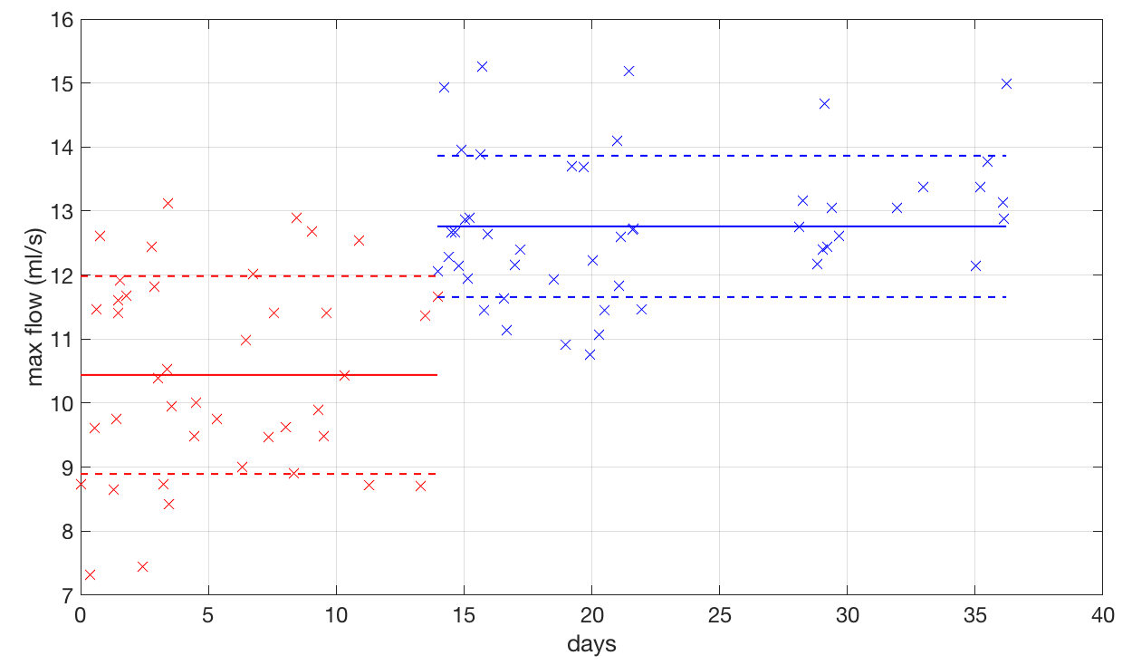 Figure 10 : Plot of max flow versus time. Red points are the results of max flow whiteout the medicine. The blue ones are the result with the medicine.
Well, as you can see, the medicine works a bit for me! The average for each situations is different and they are within more or less one standard deviation from each other. However, with this plot you can see that some times, even with the medicine, I got some low values… Those were the days I was not at my best for taking the water out of my knee. On the other hand, at some other days, even without the medicine, I was feeling like the bullet that killed Kennedy and got a good performance! In the end, statistically, I could prove that indeed the medicine was working.
Figure 10 : Plot of max flow versus time. Red points are the results of max flow whiteout the medicine. The blue ones are the result with the medicine.
Well, as you can see, the medicine works a bit for me! The average for each situations is different and they are within more or less one standard deviation from each other. However, with this plot you can see that some times, even with the medicine, I got some low values… Those were the days I was not at my best for taking the water out of my knee. On the other hand, at some other days, even without the medicine, I was feeling like the bullet that killed Kennedy and got a good performance! In the end, statistically, I could prove that indeed the medicine was working.